Pivot Table Subtotals and Grand Totals in Excel

Part of the free Module 10: Pivot Tables · Lesson 8 of 20 · Full Excel course

Updated on 5 September 2026 · Works in Excel 365, 2021, 2019 and 2016 unless noted.

Subtotals and grand totals in a pivot table are the automatic summary lines Excel adds for each group and for the report as a whole. Subtotals appear for every item of an outer row or column field; the Grand Total row and column summarise everything. Both are controlled from the Design tab and from Field Settings, and both can be moved, changed or switched off.

Table of Contents

What subtotals and grand totals actually calculate

When a pivot table holds two or more row fields, Excel inserts a subtotal line for every item of the outer field: one line per supervisor that summarises their employees, or one line per year that summarises its quarters. The Grand Total row at the bottom summarises every row and the Grand Total column on the right summarises every column when a Columns field is present.

The important detail is that neither figure is a sum of the cells you can see. Excel recalculates each total from the source records that belong to the group, so a subtotal set to Average really is the average of those records, not the average of the numbers printed above it. That single fact explains most of the surprises people have with pivot table totals.

Show, move or remove subtotals from the Design tab

Click any cell inside the pivot table so the PivotTable Analyze and Design tabs appear on the ribbon.
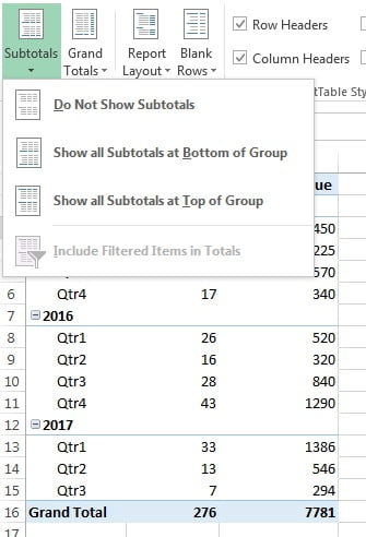
Open the Design tab and click Subtotals in the Layout group.
Choose Do Not Show Subtotals to strip every group line out of the report, leaving only the detail rows and the Grand Total.
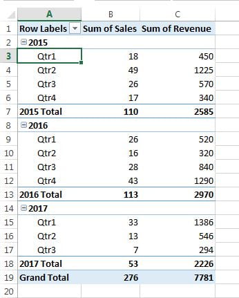
Choose Show all Subtotals at Bottom of Group to print each subtotal underneath the items it covers, on its own labelled row.
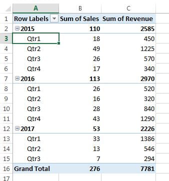
Choose Show all Subtotals at Top of Group to move the figure up onto the parent row, so the supervisor name and their total share one line.

Top of group is the compact choice and reads well on screen, because a collapsed report still shows every number. Bottom of group is the accountant’s choice and is the only option available in Tabular report layout, where the parent label already sits on the same row as the first child item. If Show all Subtotals at Top of Group looks greyed out or does nothing, switch the layout to Compact or Outline first.

Subtotals drop-down in the Layout group of the pivot table Design tab showing Do Not Show Subtotals, Show all Subtotals at Bottom of Group and Show all Subtotals at Top of Group — The Subtotals menu on the Design tab

Pivot table showing subtotals at the bottom of each group, with a labelled total row under every set of items — Subtotals at the bottom of each group

Pivot table showing subtotals at the top of each group, with the total printed on the parent row next to the item name — Subtotals at the top of each group

Turn Grand Totals on or off for rows and columns

Click inside the pivot table and open the Design tab.
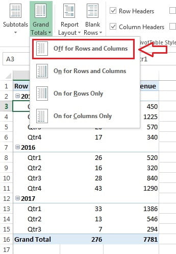
Click Grand Totals in the Layout group.
Pick the combination you need from the four options in the table below.

The wording trips almost everybody up, so read it as a description of what is being totalled rather than where the total lands.

Design > Grand Totals option	Bottom total row	Right-hand total column	Use it when
Off for Rows and Columns	Hidden	Hidden	The report feeds a chart or a dashboard tile and a total would distort the scale
On for Rows and Columns	Shown	Shown	The default; a normal cross-tab report
On for Rows Only	Shown	Hidden	Columns hold percentages or an index that must not be added across
On for Columns Only	Hidden	Shown	Each row needs its own total but a report-wide figure is meaningless

The same two switches live on the Totals & Filters tab of PivotTable Options, labelled Show grand totals for rows and Show grand totals for columns. Setting them there is handy when you are already in the dialog adjusting other behaviour, which is covered in the PivotTable Options and troubleshooting guide.

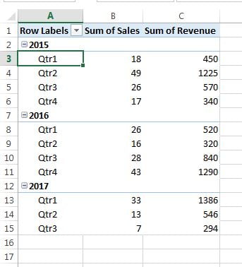
Grand Totals drop-down on the pivot table Design tab listing Off for Rows and Columns, On for Rows and Columns, On for Rows Only and On for Columns Only — The Grand Totals menu on the Design tab

Pivot table after choosing Off for Rows and Columns, with both grand total lines removed from the report — The report with Grand Totals switched off

Field Settings: Automatic, None and Custom subtotals

The Design tab is an all-or-nothing switch. To control one field on its own, right-click any item of that field and choose Field Settings, then look at the Subtotals & Filters tab.

Automatic gives one subtotal row using the same function as the value field, so Sum of Sales produces a Sum subtotal.
None removes the subtotal for this field only. Use it to keep supervisor subtotals while dropping product subtotals in the same report.
Custom unlocks the function list. Tick Sum and Average together and Excel prints two subtotal rows for every group, one labelled Sum and one labelled Average. Count, Max, Min, Product, StdDev and Var are all available, and you can tick as many as you need.

Custom subtotals are the fastest way to show a total and a per-item average side by side without adding a second value field. They only apply to fields in the Rows and Columns areas, not to fields in the Values area, whose calculation is set through Value Field Settings.

Remove a single subtotal with a right-click

You do not always need the dialog. Right-click any item of the field whose subtotal you want to lose and untick Subtotal “Field Name” at the top of the shortcut menu. The tick disappears and so does that field’s subtotal line, exactly as if you had set Field Settings to None. Right-click again and tick it back to bring it in. This is the quickest way to clean up a three-level report where only the outermost grouping deserves a total.

Include Filtered Items in Totals

The fourth entry on the Design > Subtotals menu is Include Filtered Items in Totals. When it is on, Excel adds the hidden items back into the subtotals and grand totals and marks each affected figure with an asterisk, so the report shows what one region contributed against the full company. It is greyed out for ordinary pivot tables and only becomes available when the pivot table is built on the Data Model, that is when you ticked Add this data to the Data Model while creating it or built the report from related tables. On a normal pivot table the totals always cover the filtered result only.

Worked example: why a Grand Total of Averages differs

Put Supervisor and Employee in Rows and Sales in Values, then set the Supervisor field to a Custom subtotal of Average. Five records give this picture.

Supervisor	Employee	Sales
North	Alan	120
North	Bina	80
North	Chris	100
South	Dev	60
South	Eva	40

The North average subtotal reads 100 and the South average subtotal reads 50. The average shown in the Grand Total row is 80, not 75. Excel averaged all five records (400 divided by 5), while the simple mean of the two subtotals ignores the fact that North has three employees and South only two. The Grand Total is the statistically correct number; if the business really wants an unweighted average of the two teams, calculate it outside the pivot table with =AVERAGE(100,50) or with a SUMPRODUCT weighting. The same logic applies to Count, Max, Min and to any percentage: a grand total of percentages is recalculated from the raw records, so it will rarely equal the sum of the column.

Tips and common mistakes

Subtotals need two or more fields in an area. With one row field there is nothing to group, so only the Grand Total appears.
Tabular layout refuses top-of-group subtotals. Change the layout on the Design tab first; see Report Layout: compact, outline and tabular.
Rename a total by typing over it. Click the Grand Total cell, type Company Total and press Enter. The caption survives refreshes.
Label and value filters still count in totals. On a normal pivot table the total covers the filtered items only, but a Top 10 value filter can leave a total that looks wrong beside the visible rows.
Show Values As percentages use the totals as their base. Hiding a Grand Total from view does not change the percentages, because the base is calculated internally.
Do not add a formula beside the report. A worksheet SUM next to a pivot table breaks the moment the report grows or shrinks; change the subtotal setting instead.
Blank source cells are ignored by Average. Empty cells are not treated as zero, which is another reason a subtotal can differ from what you expect.

Errors and how to fix them

Symptom	Cause	Fix
No subtotal rows anywhere	Design > Subtotals is set to Do Not Show Subtotals	Choose Show all Subtotals at Bottom of Group
One field has no subtotal, the rest do	That field is set to None in Field Settings	Right-click the field and tick Subtotal, or set Automatic
Include Filtered Items in Totals is greyed out	The pivot table is not built on the Data Model	Recreate the pivot table with Add this data to the Data Model ticked
Grand Total does not equal the visible rows	An Average, Count Distinct or percentage calculation, or a value filter	Check Value Field Settings and the active filters before assuming a bug
Grand Total column returns after a refresh	The total was deleted by hiding cells, not switched off	Use Design > Grand Totals > On for Rows Only

Practice exercise

Open the course practice file Pivot-Table.xlsx and build a pivot with Supervisor Name and Product in Rows and Sum of Sales in Values.
Move the subtotals to the top of each group, then set them back to the bottom and note which version reads better when the groups are collapsed.
Open Field Settings for Supervisor Name, choose Custom and tick Sum and Average. Confirm that two subtotal rows now appear per supervisor.
Right-click a product item and untick its Subtotal so only the supervisor level is totalled.
Switch Grand Totals to On for Rows Only, then compare the average in the Grand Total row against the simple mean of your supervisor averages.

Key takeaways

Design > Subtotals shows, moves or removes every subtotal in the report at once.
Design > Grand Totals switches the bottom row and the right-hand column independently.
Field Settings > Subtotals & Filters controls one field, and Custom can print several functions per group.
A right-click on any item lets you tick or untick that single field’s subtotal.
Include Filtered Items in Totals is a Data Model feature and stays greyed out on ordinary pivot tables.
Totals are recalculated from the source records, so a grand average is never the average of the subtotals.

Related lessons

Frequently asked questions

How do I remove the Grand Total from a pivot table?

Click inside the report, open the Design tab and choose Grand Totals, then Off for Rows and Columns. To drop only the bottom row keep On for Columns Only, and to drop only the right-hand column keep On for Rows Only. The same pair of switches sits on the Totals and Filters tab of PivotTable Options.

Why does my pivot table not show subtotals?

Either the report has a single field in the Rows area, in which case there is nothing to group, or Design > Subtotals is set to Do Not Show Subtotals, or that particular field is set to None on the Subtotals and Filters tab of Field Settings. Check the field first, because a per-field None overrides the ribbon setting.

Can one subtotal show both a sum and an average?

Yes. Right-click an item of the field, choose Field Settings, select Custom on the Subtotals and Filters tab and tick both Sum and Average. Excel then prints two labelled subtotal rows for every group while the detail rows keep the calculation set in Value Field Settings.

Why is the Include Filtered Items in Totals option greyed out?

That option only works on pivot tables built on the Data Model. Create the report again with Add this data to the Data Model ticked in the Create PivotTable dialog, or build it from related tables. On a standard pivot table the subtotals and grand totals always reflect the filtered result only.

Why is the grand total average not the average of the subtotals?

Excel averages every underlying record, not the subtotal figures. A group with ten records carries more weight than a group with two, so the grand total is a weighted average. It is the correct number for the data set; if you need an unweighted comparison of groups, calculate it outside the pivot table.

Want the finished version? Ready-made Excel dashboards, trackers and VBA systems are available at NextGenTemplates.com.