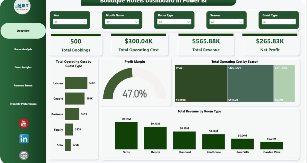
Pivot Table is useful and power full feature available in Excel. Learn the below given 10 useful Pivot table tips in Excel- Fix Column Width Running Total Ranking Move Pivot Table Report Filter Pages Pivot in PPT Conditional Formatting in Pivot Table Filter Selected Items Tabular format Repeat Labels Watch the below given video to learn all above given tips: Click here to download practice file-
In this article, you will learn about the Subtotal feature of Microsoft Excel. Excel can organize data in groups, allowing you to easily show and hide different sections of your worksheet. You can also summarize different groups using the Subtotal command and create an outline for your worksheet. To use the Subtotal feature, make sure your data is properly sorted. Here we have taken the example of Student wise marks
In this article, you will learn how to display the Progress Bar in Excel Cells. We have used Conditional Formatting Data Bar to create this. Progress Bar will be filled according to the value entered in the cell. Below are the steps to create Progress Bar in Excel Cells- Select the range for your completion percentage. Go to Home >> Conditional Formatting >> New Rule Select Format all cells based
In this article, you will learn how to use Advanced Conditional Formatting to search text in data. Here we have taken the example for employee Performance rating data. We two type of search –Search in specific column and Search in all columns. Note: This trick is useful only for small data set. Search in specific Column: To search in specific column, just select the column name form the drop down
In this article, you will learn how to add Auto Bullet Points in Excel using Custom formatting. To add the auto bullet point in excel range below are the steps- Select the excel range. Press Alt+O+E to open the Format Cells window. Go to Number tab. Got to Custom. Put the below code in Type box- “ ■ General; ■ General; ■ General; ■ General” You can take any other
In this article, you will learn how to apply the Same Chart Format on the other Charts. Let’s say we have month-wise sales data chart and we do some formatting on this, now we want to apply same formatting on day-wise sales chart. [caption id="attachment_15802" align="aligncenter" width="835"] Month-Wise Sales Chart[/caption] Below are the steps: Just copy the month-wise sales chart Select the day-wise sales Go to Home tab >> Paste
In this article, you will learn how to display hidden data on the chart. if we create a chart for month wise sales and hide or collapse few months then those months data will not be visible on the chart. [caption id="attachment_15718" align="aligncenter" width="874"] March to July data is not visible[/caption] If you want to display the hidden data on the then below are the steps- Right click on the
In this article, you will learn how to sort the data by columns. If you have multiple columns in your excel sheet and you want to arrange the order of the columns according to your requirement then you can use this trick. Let’s say we have below given data. [caption id="attachment_15653" align="aligncenter" width="827"] Data set[/caption] Now we want the arrange the columns according to our requirements. Insert a row above
Many times, when we create a chart and our numbers are quite big then our data labels on the chart are not proper readable. In that case we can change the number format of data label of the charts in millions or thousands according to our numbers. To change the number format of data labels just right click on Chart and click on Format data labels. Go to the numbers
In this article, you will learn how to get count of persons from a Date of Birth data whose birthdays are in the specific month. You will also learn how to highlight the data using Conditional Formatting whose birthdays are in This Month, Last Month and Next Month. We have below given Date of Birth data for Employees- [caption id="attachment_14951" align="aligncenter" width="435"] Date of Birth data[/caption] We have created a