Part of the free Module 10: Pivot Tables · Lesson 1 of 20 · Full Excel course
Updated on 5 September 2026 · Works in Excel 365, 2021, 2019 and 2016 unless noted.
To insert a pivot table in Excel, click one cell inside your data, go to Insert > Tables > PivotTable, confirm the range in the Create PivotTable dialog and click OK. Excel opens a blank report and the PivotTable Fields pane; drag fields into Rows, Columns, Values and Filters and the summary builds itself, with no formulas and no typing.
What a pivot table is and when to use one
A pivot table is an interactive summary report. You point it at a range or table, drag a few field names into place, and Excel groups, counts, sums or averages the data for you. Because the layout is rebuilt on every drag, you can pivot the same data from a product view to a supervisor view in seconds.
Use a pivot table whenever you need totals by category, a comparison across periods, a top-N list or a quick cross-check of a large export. It answers questions such as “Which supervisor generated the most revenue?” or “How many units of each product did we sell last month?” faster than SUMIFS or COUNTIFS formulas, and it never breaks when new rows arrive.
A pivot table is not the right tool for row-level editing, for reports that need a fixed cell layout that formulas point at, or for data that changes cell by cell every minute. For those cases use formulas or an Excel Table with structured references.
Prepare the source data first
Most pivot table problems start in the source. Check these five points before you insert anything.
| Requirement | Why it matters | How to check |
|---|---|---|
| One header row, every column named | A blank header stops Excel creating the pivot table | Look at row 1; fill any empty heading |
| No blank rows or columns inside the block | Excel stops the current region at the first empty row | Press Ctrl + A inside the data and check the selection edge |
| One data type per column | Text in a number column forces Count instead of Sum; text dates will not group | Sort the column and look at the top and bottom values |
| No total or subtotal rows | A Grand Total row in the source doubles every figure | Filter the first column for the word Total |
| No merged cells | Merged headers leave blank field names | Home > Merge & Center is not highlighted anywhere |
The best preparation is to convert the range to an Excel Table with Ctrl + T. A table has a name, expands automatically when you add rows, and the pivot table picks up those rows on refresh without you changing the data source.
Sample data used in this course
Every chapter of this Pivot Table course uses the same sales data, which you can download as the practice file Pivot-Table.xlsx. It has six columns: Date, Employee Name, Supervisor Name, Product, Sales (units) and Revenue. Each row is one transaction, the headers are in row 1 and there are no blank rows or merged cells, which is exactly the structure a pivot table needs.
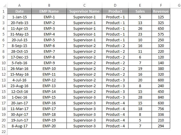
How to insert a pivot table in Excel step by step
- Click any single cell inside the data. Excel detects the current region automatically, so you do not need to select the whole range.
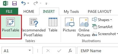
- Go to the Insert tab and, in the Tables group, click PivotTable. In Excel 365 the button is a drop-down; choose From Table/Range. The keyboard shortcut is Alt + N + V. The older Alt + D + P opens the legacy PivotTable Wizard, which still works in every version.
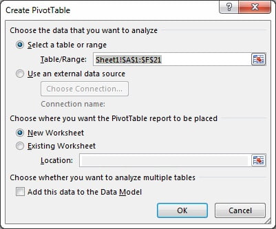
- The Create PivotTable dialog (called PivotTable from table or range in Excel 365) shows the source range or table name. Check that it covers all rows and columns.
- Choose where to place the report. Keep New Worksheet selected for a clean sheet, or pick Existing Worksheet and click a cell when you want the pivot table next to other content.
- Leave Add this data to the Data Model unticked for a normal pivot table. Tick it only when you need Distinct Count or relationships between tables, which are covered in later chapters.
- Click OK.
- An empty pivot table appears on the left and the PivotTable Fields pane opens on the right. Tick a field or drag it into one of the four areas at the bottom of the pane.
- Drag Supervisor Name to Rows, drag Sales and Revenue to Values, and drag Product to Filters. The report is ready.
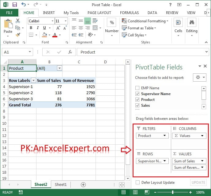
The four areas of the PivotTable Fields pane
| Area | What it does | Typical field | Default for a numeric field |
|---|---|---|---|
| Filters | Limits the whole report to one or more items shown above the table | Product, Region, Year | Not applicable |
| Columns | Spreads a field across the top of the report | Month, Product | Not applicable |
| Rows | Lists categories down the left side | Supervisor Name, Employee Name | Not applicable |
| Values | Holds the numbers being summarised | Sales, Revenue | Sum (text fields default to Count) |
A field can sit in more than one area at once. Dropping Employee Name into Values, for instance, gives a count of transactions per supervisor next to the revenue total. Ticking a text field in the list sends it to Rows; ticking a numeric field sends it to Values. Drag fields up and down inside an area to change their order, and drag a field out of the pane to remove it.
If the pane disappears, click inside the pivot table and choose PivotTable Analyze > Show > Field List. The pane can be docked, floated or widened from the small gear icon at its top right.
Recommended PivotTables and Excel 365 differences
Insert > Tables > Recommended PivotTables scans your data and offers ready-made layouts such as Sum of Revenue by Supervisor Name. Pick one and Excel builds it on a new sheet; you can then add or remove fields as usual. It is a good starting point for beginners and for unfamiliar data.
In Excel 365 the Insert > PivotTable button offers three sources: From Table/Range, From External Data Source and From Data Model. The Fields pane looks the same, and the ribbon tab is called PivotTable Analyze (it was Analyze in 2016 and 2019). Excel 365 also lets Copilot suggest a pivot table from a plain-English prompt, but the result is the same object you build by hand here.
Worked example: revenue by supervisor
Here is a cut-down version of the practice data so you can check the numbers by hand.
| Date | Employee Name | Supervisor Name | Product | Sales | Revenue |
|---|---|---|---|---|---|
| 01-Jan | Amit | Rahul | Laptop | 2 | 90,000 |
| 01-Jan | Neha | Rahul | Printer | 3 | 24,000 |
| 02-Jan | Sunil | Priya | Laptop | 1 | 45,000 |
| 02-Jan | Amit | Rahul | Mouse | 10 | 5,000 |
| 03-Jan | Kavita | Priya | Printer | 2 | 16,000 |
| 03-Jan | Sunil | Priya | Mouse | 6 | 3,000 |
Insert the pivot table with Supervisor Name in Rows and Sales and Revenue in Values. Excel produces this report:
| Row Labels | Sum of Sales | Sum of Revenue |
|---|---|---|
| Priya | 9 | 64,000 |
| Rahul | 15 | 119,000 |
| Grand Total | 24 | 183,000 |
Now put Product in Filters and choose Laptop. The report shrinks to Priya 1 unit and 45,000, Rahul 2 units and 90,000. That is the whole idea: the same six rows answer a new question every time you move a field.
Tips and common mistakes
- One header per column. A blank header stops the pivot table being created, and a duplicate header is silently renamed with a number.
- Keep one data type per column. Dates stored as text will not group by month, and numbers stored as text are counted instead of summed.
- Remove totals from the source. A Grand Total row in the raw data doubles every figure in the pivot table.
- Pivot tables do not update by themselves. After editing the source, right-click the report and choose Refresh, or press Alt + F5.
- Do not type inside the pivot table. The report is read-only. Change the source data and refresh instead.
- Use a Table as the source. A plain range is frozen at its original size; a Table grows with the data.
- Rename value headings. Click the heading cell and type a new name such as Total Revenue. Excel refuses a name identical to the source field, so add a space or a word.
Errors and how to fix them
| Problem | Cause | Fix |
|---|---|---|
| The PivotTable field name is not valid | A header cell in the source is blank | Type a heading in every column of row 1 and try again |
| The pivot table shows only part of the data | A blank row or column split the current region | Delete the blank row, or select the full range before inserting |
| Values show Count of Revenue instead of Sum | Text or blank cells in the Revenue column | Convert the column to numbers, refresh, then set Sum in Value Field Settings |
| Dates appear as individual days and will not group | Dates stored as text | Convert with Data > Text to Columns or DATEVALUE, then refresh |
| New rows are missing after refresh | Source is a fixed range, not a Table | Press Ctrl + T on the source or use PivotTable Analyze > Change Data Source |
| PivotTable button is greyed out | Workbook is shared or protected, or the sheet is protected | Unshare or unprotect the workbook and sheet |
Practice exercise
Open the practice file Pivot-Table.xlsx and complete these tasks.
- Convert the data to an Excel Table with Ctrl + T, then insert a pivot table on a new worksheet showing Sum of Revenue by Supervisor Name.
- Add Product to Columns so each supervisor’s revenue is split by product. Note which product has the highest grand total.
- Move Product from Columns to Filters and switch the report to one product at a time.
- Drag Employee Name to Values. Check that it shows Count of Employee Name, then rename the heading to Transactions.
- Add a new row to the source table, refresh the pivot table with Alt + F5 and confirm the totals change.
Key takeaways
- Insert a pivot table with one click in the data, then Insert > Tables > PivotTable (Alt + N + V) > OK.
- Source data needs one header row, no blank rows, one data type per column and no total rows.
- Rows, Columns, Values and Filters are the four areas; numeric fields default to Sum and text fields to Count.
- Convert the source to a Table with Ctrl + T so new rows arrive on refresh.
- Pivot tables are read-only summaries; edit the source and press Alt + F5.
Related lessons
- Pivot Table course hub
- Sort data in a pivot table
- Value Field Settings: Sum, Average, Count and Show Values As
- Refresh a pivot table and change its data source
- Distinct Count with the Data Model
- Sort and Filter module
- SUMIFS function for formula-based summaries
- Microsoft Support: Create a PivotTable to analyze worksheet data
Frequently asked questions
Where is the PivotTable option in Excel?
It is on the Insert tab, in the Tables group at the far left of the ribbon. The shortcut Alt + N + V opens the same dialog. In Excel 365 the button is a drop-down with From Table/Range as the first choice, and Insert > Recommended PivotTables lets Excel suggest a layout for you.
What data do I need to create a pivot table?
A block of data with a single header row, one record per row, no blank rows or columns, no merged cells and no total rows. Each column should hold one type of value: dates as real dates, amounts as numbers. Convert the block to an Excel Table with Ctrl + T so the pivot table grows with it.
Can I create a pivot table from multiple sheets?
Yes. Format each sheet as a Table, tick Add this data to the Data Model in the Create PivotTable dialog and relate the tables on a common column, or combine the sheets first with Power Query and pivot the result. Chapter 18 of this course walks through the Data Model method.
Why does my pivot table show Count instead of Sum?
The column contains at least one text value or blank cell, so Excel treats the whole field as text and counts it. Clean the column, convert numbers stored as text, refresh the pivot table and then change the calculation to Sum in Value Field Settings.
What is the keyboard shortcut to insert a pivot table?
Press Alt + N + V in Excel 2016 and later; in Excel 365 follow it with T for From Table/Range. The legacy shortcut Alt + D + P opens the three-step PivotTable and PivotChart Wizard, which also allows multiple consolidation ranges. Alt + F5 refreshes the selected pivot table afterwards.
Want the finished version? Ready-made Excel dashboards, trackers and VBA systems are available at NextGenTemplates.com.