Sort Data in a Pivot Table by Values or Labels

Part of the free Module 10: Pivot Tables · Lesson 2 of 20 · Full Excel course

Updated on 5 September 2026 · Works in Excel 365, 2021, 2019 and 2016 unless noted.

To sort data in a pivot table, right-click a value cell, point to Sort and choose Sort Largest to Smallest; to sort labels, open the Row Labels drop-down and pick Sort A to Z. Excel stores the sort with the field, so the order survives refreshes, filters and layout changes. This lesson covers value sorts, label sorts, manual drag order and custom lists.

Why sort inside the pivot table and not the source

The order of the raw data has no effect on a pivot table. Excel arranges row and column items alphabetically (A to Z) by default and recalculates that order every time you refresh. Sorting inside the pivot table is therefore the only reliable way to rank supervisors by revenue, list priorities as Low, Medium, High, or push a Not Assigned item to the bottom.

A pivot table sort is a property of the field, not of the cells. When you sort Supervisor Name by Sum of Revenue, Excel remembers “sort this field descending by that value field” and reapplies the rule after every refresh. That is different from Data > Sort on a normal range, which rearranges cells once and forgets.

Four ways to sort a pivot table compared

Method	Where to click	Sorts by	Best for
Value sort	Right-click a number > Sort > Largest to Smallest	The value column you clicked	Rankings and leaderboards
Label sort	Row Labels drop-down > Sort A to Z or Z to A	The text, date or number in the label	Alphabetical lists, date order
Manual sort	Drag the item, or right-click > Move	Your own arrangement	Small lists with a business order
Custom list	File > Options > Advanced > Edit Custom Lists, then Sort A to Z	The sequence in the list	Low/Medium/High, regions, month names stored as text

How to sort a pivot table by values (largest to smallest)

We continue with the supervisor-wise pivot table from the previous chapter and want the supervisor with the highest revenue at the top.

Right-click any number in the Sum of Revenue column. Do not right-click the header, because that sorts the row labels instead.
Point to Sort in the shortcut menu and click Sort Largest to Smallest. Choose Sort Smallest to Largest for the reverse order.

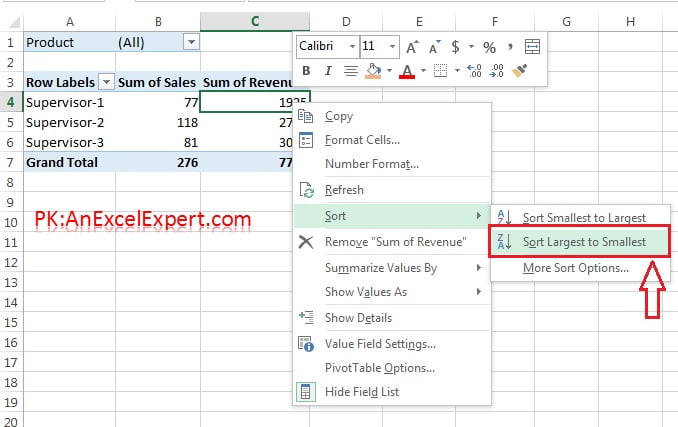
Right-click Sort menu on the Sum of Revenue column used to sort data in a pivot table largest to smallest — Right-click, Sort, Sort Largest to Smallest

The rows are rearranged instantly. The supervisor with the highest revenue is now first and the Grand Total row stays fixed at the bottom.

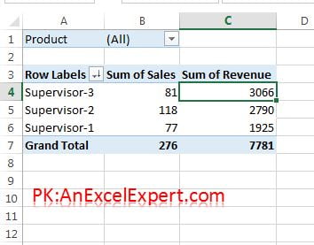
Pivot table sorted by Sum of Revenue in descending order with the highest supervisor at the top — Pivot table sorted by Revenue in descending order

You can get the same result from the ribbon: select a value cell and click Data > Sort & Filter > Sort Z to A. Or open the Row Labels drop-down, choose More Sort Options, pick Descending (Z to A) by and select Sum of Revenue from the list. The More Sort Options dialog is the only place that shows you which value field a label field is currently sorted by.

Sort row or column labels

Click the drop-down arrow on Row Labels (or Column Labels) and choose Sort A to Z or Sort Z to A. When the report has several row fields, the drop-down has a Select field box at the top; pick the field you want before choosing the order. Dates and numbers used as labels sort chronologically or numerically, not as text, as long as they are real dates and numbers in the source.

In compact layout the Row Labels heading is shared by all row fields. To sort an inner field, right-click one of its items instead and use Sort from the shortcut menu.

Sort a cross-tab by one column or one row

When Product sits in Columns and Supervisor Name in Rows, right-clicking a value in the Laptop column and choosing Sort Largest to Smallest ranks the supervisors by laptop revenue only. Excel confirms this in More Sort Options: open it and the Summary box reads “Sort Supervisor Name by Sum of Revenue in descending order using values in this column: Laptop”.

To sort the column items (Products) by one supervisor’s numbers, right-click a value in that supervisor’s row and sort. If Excel picks the wrong direction, open More Sort Options > More Options, choose Values in selected row or Values in selected column, and click the cell reference you want to use.

Manual sort by dragging

Select a row label, hover over the cell border until the four-headed arrow appears and drag the item to a new position. Alternatively right-click the item, point to Move and choose Move Up, Move Down, Move to Beginning or Move to End. The field switches to Manual sort order automatically, which you can confirm in More Sort Options. A manual order is kept on refresh; new items that appear after a refresh are added at the end.

Sort by a custom list

If your labels are text such as Low, Medium, High, Excel would sort them High, Low, Medium alphabetically. Create a custom list instead.

Go to File > Options > Advanced, scroll to the General section and click Edit Custom Lists.
Type the items in order, one per line (Low, Medium, High), click Add, then OK twice.
In the pivot table open the field drop-down and choose Sort A to Z. Excel now follows the list.

Pivot tables use custom lists only while Use Custom Lists when sorting is ticked under PivotTable Options > Totals & Filters. It is on by default. Untick it when you want month names such as Jan and Feb to sort alphabetically instead of by calendar, or when a built-in day-name list is interfering with a text field.

Worked example: rank employees within each supervisor

Put Supervisor Name and then Employee Name in Rows with Sum of Revenue in Values. Before sorting, the report lists everyone alphabetically:

Row Labels	Sum of Revenue
Priya	64,000
Kavita	16,000
Sunil	48,000
Rahul	119,000
Amit	95,000
Neha	24,000

Right-click Kavita’s 16,000 and choose Sort > Sort Largest to Smallest. Only the inner field changes: Sunil moves above Kavita and Amit stays above Neha, while the supervisor order is untouched. Now right-click Priya’s 64,000 subtotal and sort largest to smallest again. Rahul moves to the top because the outer field is now ranked by its own subtotal.

Row Labels	Sum of Revenue
Rahul	119,000
Amit	95,000
Neha	24,000
Priya	64,000
Sunil	48,000
Kavita	16,000

Each field keeps its own sort rule, so you can rank supervisors by revenue and employees by sales units if you prefer.

Tips and common mistakes

Sorting the wrong field. Right-clicking a label sorts the labels; right-clicking a value sorts by that value. Watch which column you click.
Months sorting alphabetically. This happens when month names are text in the source. Use real dates and let the pivot table group them, or apply a custom list.
Sort lost after refresh. Open More Sort Options > More Options and untick Sort automatically every time the report is updated if you want to keep an arrangement. Ticked is the default and is usually what you want for value sorts.
Sorting a chart instead of the table. Pivot charts follow the pivot table order, so always sort the table, never the chart.
Grand Total row will not move. Totals are always last. If you want a total at the top, add a second Values field with Show Values As set to % of Grand Total instead.
Data > Sort dialog is greyed out. The full Sort dialog does not work inside a pivot table. Use the right-click menu or More Sort Options.
Manual order goes back to A to Z. Choosing Sort A to Z from the drop-down cancels the manual order. Use Move commands to fine-tune instead.

Errors and how to fix them

Problem	Cause	Fix
Sort options are missing from the right-click menu	You right-clicked a blank cell or the Grand Total label	Right-click a data value or a row item
Items sort as 1, 10, 2 instead of 1, 2, 10	Numbers stored as text in the source	Convert with Data > Text to Columns, refresh, sort again
Jan, Feb, Mar sort as Feb, Jan, Mar	Use Custom Lists when sorting is off, or names have spaces	Tick the option in PivotTable Options > Totals & Filters, or group real dates
Sort changes when a filter is applied	Automatic sort recalculates on the visible values	Expected; use manual sort if the order must be fixed
New item appears in the wrong place	Field is in manual sort order	Drag the item, or switch back to Ascending in More Sort Options

Practice exercise

Open the practice file Pivot-Table.xlsx and build an employee-wise pivot table with Sum of Sales and Sum of Revenue.

Sort the employees largest to smallest by Revenue and note the top three.
Sort them smallest to largest by Sales and compare: does the ranking change?
Add Product to Columns and sort the employees by one product only. Open More Sort Options and read the Summary box.
Create a custom list of the product names in your preferred order and sort the Product column labels A to Z.
Drag one employee to the top manually, refresh the pivot table with Alt + F5 and confirm the order stays.

Key takeaways

Right-click a value to sort by numbers; use the Row Labels drop-down to sort by labels.
A pivot table sort is a rule stored on the field and is reapplied on every refresh.
In a cross-tab, the column you right-click decides which values drive the sort.
Drag or use Move commands for a manual order; custom lists handle Low, Medium, High.
More Sort Options shows and controls exactly how each field is sorted.

Related lessons

Frequently asked questions

How do I sort a pivot table by the Grand Total column?

Right-click any value in the Grand Total column and choose Sort > Sort Largest to Smallest. The row items are ranked by their overall total while the column order stays unchanged. Open More Sort Options if you want to confirm that the Summary box says the sort uses the Grand Total column.

Why can I not sort my pivot table?

The field is usually in manual sort order, the sheet is protected, or you right-clicked a blank or total cell. Open the Row Labels drop-down, choose More Sort Options and pick Ascending or Descending to switch back to automatic sorting, then right-click a real value and sort again.

Can I sort a pivot table by two columns at once?

A single field can be sorted by only one value field at a time. To rank by Revenue and then by Sales, sort the outer field by Revenue and the inner field by Sales, or add a helper column in the source that combines both, such as Revenue plus Sales divided by 1,000,000, and sort by that.

How do I sort months in the correct order in a pivot table?

Keep the dates as real dates in the source and group them by month inside the pivot table; grouped months always sort by calendar. If the source already holds month names as text, make sure Use Custom Lists when sorting is ticked in PivotTable Options and the names match Excel’s built-in Jan to Dec list.

Does the pivot table sort stay after a refresh?

Yes. The sort is stored with the field and reapplied automatically. If you would rather freeze the current arrangement, open More Sort Options > More Options and untick Sort automatically every time the report is updated, or switch to manual sort by dragging an item.

Want the finished version? Ready-made Excel dashboards, trackers and VBA systems are available at NextGenTemplates.com.