Pivot Table Report Layout: Compact, Outline and Tabular Form

Part of the free Module 10: Pivot Tables · Lesson 7 of 20 · Full Excel course

Updated on 5 September 2026 · Works in Excel 365, 2021, 2019 and 2016 unless noted.

The pivot table report layout decides how row fields are arranged on the sheet. Compact form stacks every row field in one indented column, Outline form gives each field its own column with subtotals above the group, and Tabular form gives each field its own column with subtotals below. All three show identical numbers; only the shape changes.

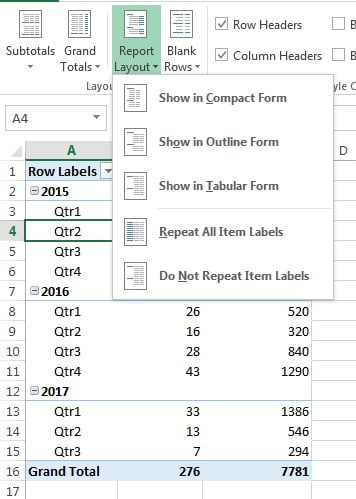
Where to find Report Layout

Click any cell inside the pivot table, then open the Design tab, called PivotTable Design in Excel 365 and on the Mac, and click Report Layout in the Layout group. Five commands appear.

• Show in Compact Form, Show in Outline Form and Show in Tabular Form are mutually exclusive. Choosing one switches off the other two.
• Repeat All Item Labels and Do Not Repeat Item Labels are a separate on or off switch that works in Outline and Tabular form only.

The change applies to the whole pivot table at once and survives a refresh, so you set it once per report rather than every time the data updates.

Compact form, the default layout

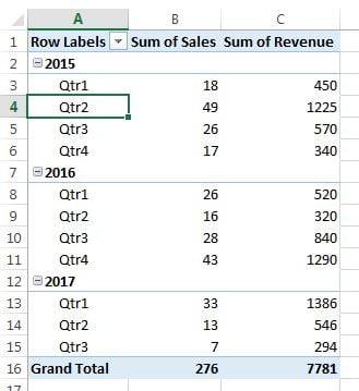
In Compact form every row field shares one column and each inner level is indented under its parent. The column header reads Row Labels rather than the real field names, and a single expand or collapse button controls the whole hierarchy.

Compact form uses the least horizontal space, which is why Excel applies it to every new pivot table. It reads well on screen and prints well when the report is deep rather than wide. The weakness is that the row field values sit in one column, so the output cannot be filtered, sorted or looked up as a flat list.

Outline form

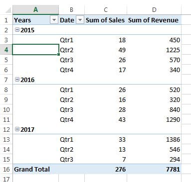
Outline form gives every row field its own column and puts the real field name in the header. Subtotals stay at the top of each group, on the same line as the parent item, and the child items are listed underneath. The indented look of Compact form is preserved, but the headers now say what each column actually contains.

Use Outline form when a reader needs to see the group total before the detail, which is the way most management reports are read. It also suits printing with Repeat item labels switched off, because each group is announced clearly by its own heading row.

Tabular form

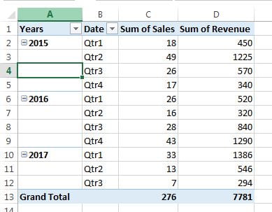
Tabular form also gives every field its own column, but the first child item sits on the same row as its parent and the subtotal moves to the bottom of the group. Nothing is indented, so the report looks like a traditional spreadsheet table.

This is the layout to choose when the pivot output will be reused: copied and pasted as values, referenced by a lookup formula, loaded into Power Query, or sent to someone who will open it in another tool. It is also the only layout in which every row field has a genuine header cell that a lookup can point at.

Compact, Outline and Tabular compared

Feature	Compact form	Outline form	Tabular form
Row fields	All in one column, indented	One column each	One column each
Column header	Row Labels	Real field name	Real field name
Subtotal position	Top of group	Top of group	Bottom of group
First child item	New indented row	New row below the parent	Same row as the parent
Width used	Narrowest	Medium	Widest
Repeat All Item Labels	Not available	Available	Available
Expand and collapse buttons	Yes, on the single column	Yes, per field	Yes, per field
Best for	Reading on screen, deep hierarchies	Printed management reports	Exporting, lookups, Power Query

Repeat All Item Labels and why it matters

By default an outer field value is printed once, on the first row of its group, and the cells below it are blank. That reads nicely but it is not a dataset. Turn the labels back on in three clicks.

1. Click any cell inside the pivot table.
2. Choose Design > Report Layout > Show in Tabular Form.
3. Open Report Layout again and choose Repeat All Item Labels. Every row now carries its own outer field value.

Choose Do Not Repeat Item Labels to go back. Tabular form plus repeated labels is the export format: it is what VLOOKUP, XLOOKUP, SUMIFS, COUNTIFS, a second pivot table, Power Query and Power BI all expect. Every one of those breaks on blank key cells, because a lookup on a blank returns the wrong row or an error rather than the value you meant.

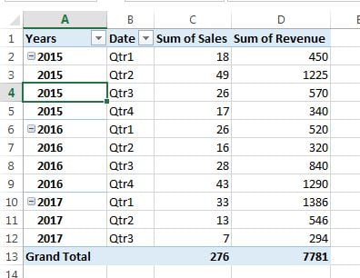
Blank Rows between groups

Next to Report Layout sits Design > Layout > Blank Rows, with two commands: Insert Blank Line after Each Item and Remove Blank Line after Each Item. The blank line separates groups visually in Outline and Tabular form and is genuinely useful on a long printed report.

Treat it as presentation only. The blank line is part of the pivot table, so it is copied with the report and it will confuse anything that reads the result as data. Remove it before you paste values, and never combine it with Repeat All Item Labels on a range you intend to feed into a lookup.

Per-field layout in Field Settings

The Design tab applies one layout to the entire report. Field Settings lets you override that for a single field, which is how you build a hybrid such as tabular outer fields with a compact inner field.

1. Right-click any item of the field, or click the field in the Rows box of the Fields pane, and choose Field Settings.
2. Open the Layout & Print tab.
3. Under Layout, pick Show item labels in outline form or Show item labels in tabular form. Outline form adds the two extra options below it: Display labels from the next field in the same column (compact form) and Display subtotals at the top of each group.
4. Tick Repeat item labels to repeat this one field only, and Insert blank line after each item label for a gap after this field only.
5. Under Print, tick Insert page break after each item if each group should start a new printed page.

Because these settings live on the field, they survive a refresh and a change of data source. Untick Display labels from the next field in the same column on a compact report and that field alone moves into its own column.

Setting the default layout for every new pivot table

In Excel 2019 and Excel 365 you can stop switching layouts by hand and change what Excel does on creation. Go to File > Options > Data and click Edit Default Layout. Set Report Layout to Show in Tabular Form, set Subtotals and Grand Totals as you prefer, and tick Repeat All Item Labels if you build exports more often than presentations.

The dialog also has an Import button: click a pivot table you have already formatted, then click Import, and Excel copies its layout as the new default. The PivotTable Options button opens the full options dialog so defaults such as autofit and preserve formatting can be set at the same time. This is a per-user Excel setting, so it applies to every workbook you create on that machine and to nobody else. Excel 2016 has no Edit Default Layout button; there you set the layout on each pivot table, or keep a formatted pivot table in a template workbook.

Worked example

Open the course practice file and build a pivot with Supervisor Name and Employee Name in Rows and Sum of Revenue in Values. Compact form gives you something like this, with the two fields sharing one column.

Row Labels	Sum of Revenue
Supervisor A	48,200
Agent 1	21,500
Agent 2	26,700
Supervisor B	33,900

Now choose Design > Report Layout > Show in Tabular Form and then Repeat All Item Labels. The same numbers arrive as a flat list with the supervisor on every line and the subtotal moved below the group.

Supervisor Name	Employee Name	Sum of Revenue
Supervisor A	Agent 1	21,500
Supervisor A	Agent 2	26,700
Supervisor A Total		48,200
Supervisor B	Agent 3	33,900

Copy the range, paste it on a blank sheet with Paste Special > Values, delete the total rows, and you have a clean two-key table that =XLOOKUP(A2,...) or =SUMIFS(...) can read directly.

Tips and common mistakes

• Repeat All Item Labels is greyed out. You are still in Compact form. The command only works in Outline or Tabular form, so switch layout first.
• Do not paste a pivot table straight into a lookup range. Turn on repeated labels, remove blank rows, remove subtotals with Design > Subtotals > Do Not Show Subtotals, then paste as values.
• Layout is not formatting. Report Layout moves fields; pivot table styles change colours and banding. Changing the layout does not disturb the style you picked.
• Watch the width. Tabular form adds one column per row field, so a five-field report suddenly needs five columns before the first number.
• Missing expand and collapse buttons. Switch them back on with PivotTable Analyze > Show > +/- Buttons.
• Column widths keep resetting. That is autofit, not the layout. Untick Autofit column widths on update in PivotTable Options.
• One report, one layout. If a colleague needs both shapes, build a second pivot table from the same source rather than switching back and forth.

Practice exercise

1. Build a pivot with two row fields and one value field, then apply each of the three layouts in turn and write down where the subtotal appears in each one.
2. Switch to Tabular form, turn on Repeat All Item Labels, and confirm no cell in the outer field column is blank.
3. Use Design > Blank Rows > Insert Blank Line after Each Item, print preview the report, then remove the blank lines again.
4. Open Field Settings > Layout & Print for the inner field only and set it to outline form while the outer field stays tabular.
5. Set File > Options > Data > Edit Default Layout to Tabular, then insert a brand-new pivot table and check it starts in the layout you chose.

Key takeaways

• Compact, Outline and Tabular form change the shape of the report, never the numbers.
• Compact form saves space; Outline form adds field headers with subtotals on top; Tabular form is flat with subtotals below.
• Tabular form plus Repeat All Item Labels is the format to use whenever the output feeds a lookup, Power Query or another system.
• Blank Rows is presentation only and should be removed before the result is reused as data.
• Field Settings on the Layout & Print tab overrides the layout for a single field.
• Excel 2019 and 365 can make your preferred layout the default through File > Options > Data > Edit Default Layout.

Related lessons

• Columns in a pivot table: building cross-tab reports
• Subtotals and Grand Totals in a pivot table
• Pivot table, slicer and timeline styles
• PivotTable Options, settings and troubleshooting
• Pivot Table course hub
• VLOOKUP function and the Excel Dashboard module
• Microsoft Support: Create a PivotTable to analyse worksheet data

Frequently asked questions

Which pivot table report layout is best?

It depends on the reader. Compact form is best on screen because it is narrowest. Outline form suits printed management reports, since every field is headed and the group total sits above the detail. Tabular form with repeated item labels is best whenever the result will be copied, looked up, sorted or loaded into Power Query.

How do I show the real field names instead of Row Labels?

Row Labels is the header Compact form uses because several fields share one column. Switch to Design > Report Layout > Show in Outline Form or Show in Tabular Form and each row field moves into its own column carrying its own field name in the header cell.

Why is Repeat All Item Labels greyed out?

The command is disabled in Compact form, where the outer values are indentation rather than a column of their own. Apply Outline or Tabular form first and it becomes available. You can also repeat a single field by ticking Repeat item labels in Field Settings on the Layout and Print tab.

Does changing the report layout affect the numbers?

No. Layout controls only how row fields are positioned and where subtotals are printed. The values, filters, sorting and calculations are untouched, so you can switch layouts freely on a finished report and switch back without recalculating or refreshing anything.

How do I make Tabular form the default for new pivot tables?

In Excel 2019 and Excel 365 go to File > Options > Data and click Edit Default Layout, then set Report Layout to Show in Tabular Form. Use the Import button to copy the settings from a pivot table you have already formatted. Excel 2016 has no such option.

Want the finished version? Ready-made Excel dashboards, trackers and VBA systems are available at NextGenTemplates.com.