Value Field Settings in Pivot Table: Sum, Average, % Share

Part of the free Module 10: Pivot Tables · Lesson 4 of 20 · Full Excel course

Updated on 5 September 2026 · Works in Excel 365, 2021, 2019 and 2016 unless noted.

Value Field Settings is the pivot table dialog that decides how each number in the Values area is calculated and displayed. Its Summarize Values By tab switches Sum to Average, Count, Max or Min, and its Show Values As tab turns the same figure into a percentage, a running total, a difference or a rank without a single worksheet formula.

What Value Field Settings controls

Every field you drop into the Values area gets a default calculation. Excel uses Sum when the column is entirely numeric and Count when it contains text or blank cells. Value Field Settings is where you override that default, rename the column heading and lock in a number format that survives a refresh.

Open it in any of three ways: right-click a value cell and choose Value Field Settings, click the field’s drop-down in the Values area of the PivotTable Fields pane, or select a value cell and use PivotTable Analyze > Active Field > Field Settings. The dialog has two tabs, and understanding the split between them is the whole lesson: Summarize Values By changes the maths, Show Values As changes the presentation of that maths.

Summarize Values By: every aggregation compared

These functions all work on the underlying source rows behind each cell, never on the numbers you can see on screen. That is why a pivot Average is a true average of every transaction rather than an average of the subtotals above it.

Summarise by	What it returns	Typical use
Sum	Total of the numeric values	Revenue, quantity, hours
Count	Number of non-blank cells, text included	Number of transactions or orders
Count Numbers	Number of numeric cells only	How many rows actually carry a figure
Average	Mean of the numeric values	Average order value, average score
Max / Min	Largest and smallest value	Biggest single sale, earliest date
Product	All values multiplied together	Compounded growth factors
StdDev / StdDevp	Standard deviation of a sample or a population	Spread of results, quality control
Var / Varp	Variance of a sample or a population	Statistical analysis
Distinct Count	Number of unique items	How many different customers bought

Distinct Count is the one entry that is not always available. It appears only when the pivot table is built on the Data Model, which you enable by ticking Add this data to the Data Model in the Create PivotTable dialog. See distinct count in a pivot table for the full method.

How to change Sum to Average in a pivot table

The example below starts from the supervisor-wise pivot table and converts Sum of Revenue into Average of Revenue.

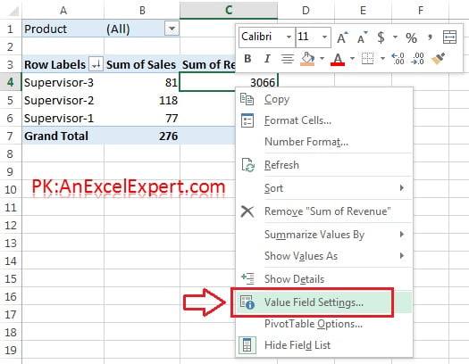
1. Right-click any cell inside the Sum of Revenue column and click Value Field Settings.

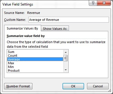
2. On the Summarize Values By tab, select Average in place of Sum. The Custom Name box at the top changes to Average of Revenue. Edit it to something shorter such as Avg Revenue if the column heading is too wide.
3. Click Number Format at the bottom left, pick Number with two decimal places or Currency, and click OK. A format set here belongs to the field, so it survives refreshes and layout changes.

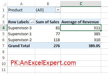
4. Click OK. Each supervisor now shows the average revenue per transaction, and the Grand Total shows the overall average of every row rather than a sum or an average of the subtotals.

Show Values As: percentages, running totals and ranks

The second tab keeps the aggregation you chose and recalculates how it is displayed relative to other cells. You can also reach it directly by right-clicking a value cell and pointing to Show Values As. Several options ask for a Base field (which field to compare across) and some also ask for a Base item (which member of that field is the benchmark).

Show Values As	Result	Base field needed	Best for
% of Grand Total	Each cell divided by the grand total	No	Share of total revenue
% of Column Total	Each cell divided by its column total	No	Product mix inside each region
% of Row Total	Each cell divided by its row total	No	How a supervisor splits across quarters
% Of	Cell compared with one chosen item	Field and item	Everything indexed to a baseline product
% of Parent Row Total	Cell divided by its outer row subtotal	No	Employee share of the supervisor total
% of Parent Column Total	Cell divided by its outer column subtotal	No	Nested column hierarchies
% of Parent Total	Cell divided by the parent in a chosen field	Field	Custom hierarchy shares
Difference From	Cell minus the base item	Field and item	Month on month change in units
% Difference From	Change expressed as a percentage	Field and item	Growth rate versus previous period
Running Total In	Cumulative total down the base field	Field	Year to date revenue
% Running Total In	Cumulative share, ending at 100%	Field	Pareto or ABC analysis
Rank Smallest to Largest	Rank 1 for the lowest value	Field	Worst performers first
Rank Largest to Smallest	Rank 1 for the highest value	Field	League table of employees
Index	Relative weight against row and column totals	No	Spotting over-indexed segments

For a percentage of the grand total, right-click the value column, point to Show Values As and click % of Grand Total. For a difference, choose % Difference From, set the base field to your grouped Date field and set the base item to (previous). For a cumulative column, choose Running Total In and pick the field that runs down the rows.

The trick that makes this practical is adding the same field to the Values area twice. Drag Revenue in a second time, leave the first copy as Sum and set the second to % of Grand Total, then rename both in Custom Name. One column gives the amount, the next gives the share.

Worked example: a four column sales report

Take a short extract of the practice data.

Product	Revenue
Product – 1	60,000
Product – 2	30,000
Product – 3	10,000

Put Product in Rows and drag Revenue into Values four times. Leave copy one as Sum and rename it Revenue Total. Set copy two to Average and name it Avg Order. Set copy three to % of Grand Total and name it Share. Set copy four to Rank Largest to Smallest with Product as the base field and name it Rank. The result reads: Product – 1 gets 60% and rank 1, Product – 2 gets 30% and rank 2, Product – 3 gets 10% and rank 3. Nothing on the worksheet has changed and every column refreshes with the data.

Tips and common mistakes

• Format inside the dialog, not on the sheet. Cell formatting is lost when the layout changes or the pivot refreshes. The Number Format button in Value Field Settings is permanent.
• A custom name cannot equal the field name. Excel rejects Revenue as a heading because the source field is called Revenue. Add a trailing space or write Total Revenue.
• Averages are never averaged. Subtotals and grand totals recalculate from the source rows, so an Average grand total will not match the mean of the visible rows.
• Show Values As replaces the number. If you need the amount as well, add the field to Values a second time instead of converting the only copy.
• Difference From leaves the first row blank. With base item (previous) the earliest period has nothing to compare against, which is correct rather than a bug.
• Running totals need a sorted base field. Sort dates or categories in the intended order first, otherwise the cumulative column runs in the wrong sequence.
• Show Values As only compares what is visible. Filters change the grand total, so percentages recalculate whenever you slice the report.

Errors and how to fix them

What you see	Cause	Fix
Count of Revenue instead of Sum of Revenue	Text, spaces or blanks in the source column	Clean the column, refresh, then set Sum in Value Field Settings
Distinct Count is greyed out	The pivot is not built on the Data Model	Recreate the pivot with Add this data to the Data Model ticked
Percentages all show 100%	% of Row Total on a report with a single value column	Switch to % of Grand Total or % of Column Total
#N/A in a Difference From column	The base item does not exist for that row	Use (previous) or (next) as the base item
Number format resets after refresh	The format was applied to cells	Reapply it through the Number Format button in the dialog

Practice exercise

1. Open the course practice file Pivot-Table.xlsx and build a supervisor-wise pivot with Revenue in Values.
2. Change the calculation to Average, rename the column Avg Revenue and set a currency format with no decimals.
3. Add Revenue a second time and set it to % of Grand Total. Confirm the percentages add up to 100%.
4. Add Revenue a third time as Rank Largest to Smallest with Supervisor as the base field.
5. Group Date by month, add a fourth copy set to % Difference From with base field Date and base item (previous), and read off the monthly growth rate.

Key takeaways

• Summarize Values By changes the calculation, Show Values As changes how that calculation is presented.
• Aggregations always run on the source rows, which is why grand totals are recalculated and not added up.
• Adding the same field to Values several times is the standard way to show amount, share and rank together.
• Number formats and custom names belong in the dialog so they survive a refresh.
• Distinct Count requires a Data Model pivot table.

Related lessons

• Pivot Table course hub
• Calculated field and calculated item for maths that Value Field Settings cannot do
• Distinct count with the Data Model
• GETPIVOTDATA to pull these values into a dashboard
• Columns in a pivot table and subtotals and grand totals
• Excel Dashboard module and the SUMIFS function as the formula alternative
• Microsoft reference: Show different calculations in PivotTable value fields

Frequently asked questions

How do I show a percentage in a pivot table?

Right-click a cell in the value column, point to Show Values As and choose % of Grand Total, % of Column Total or % of Row Total. If you want the amount and the percentage side by side, drag the same field into the Values area twice and convert only the second copy.

Why is my pivot table counting instead of summing?

At least one cell in the source column holds text, a space or a blank, so Excel treats the whole field as text and defaults to Count. Clean the column, refresh the pivot table, then open Value Field Settings and select Sum. Converting the column to a proper number format first prevents it recurring.

What is the difference between Count and Count Numbers?

Count returns the number of non-blank cells, text included, which matches the COUNTA worksheet function. Count Numbers returns only cells holding numeric values, matching COUNT. Use Count for a transaction count and Count Numbers when you need to know how many rows actually carry a figure.

How do I add a running total to a pivot table?

Add the field to Values, open Show Values As and choose Running Total In, then pick the base field that runs down the rows, usually a grouped Date field. Sort that field in the intended order first, because the cumulative figure follows the display sequence rather than the calendar.

Why is Distinct Count missing from my pivot table?

Distinct Count only exists in pivot tables built on the Data Model. Delete the pivot, insert it again and tick Add this data to the Data Model in the Create PivotTable dialog. Distinct Count then appears at the bottom of the Summarize Values By list.

Want the finished version? Ready-made Excel dashboards, trackers and VBA systems are available at NextGenTemplates.com.