Group Dates, Numbers and Text in a Pivot Table in Excel

Part of the free Module 10: Pivot Tables · Lesson 6 of 20 · Full Excel course

Updated on 5 September 2026 · Works in Excel 365, 2021, 2019 and 2016 unless noted.

To group dates in a pivot table, right-click any date in the report, click Group, and tick Months, Quarters or Years in the Grouping dialog. The same command bands numbers into ranges and merges selected text items into one category. Grouping lives inside the pivot table, so your source data is never changed.

What grouping does and when to use it

Raw transaction data is normally too granular to report on. A year of sales holds 365 possible dates, and every one of them becomes a row in the pivot table. Grouping collapses those rows into the levels a manager actually reads: month, quarter or year. It does the same job for numbers, turning order values into bands such as 0 to 4,999 and 5,000 to 9,999, and for text, letting you fold four products into two categories without adding a helper column to the source.

Because a group is stored in the pivot cache and not in the worksheet, you can create it, change it and remove it as often as you like. The table below shows what each field type supports.

Field type	Grouping method	Dialog name	Typical result
Date or date and time	Automatic, or right-click and Group	Grouping (Seconds to Years)	Years, Quarters, Months, Days
Number	Right-click a value and Group	Grouping (Starting at, Ending at, By)	Equal-width bands such as 0-4999
Text	Select two or more items, right-click and Group	None, groups are built by hand	Group1, Group2 which you then rename
Data Model field	Text grouping only in Excel 2016 and later	None	Date grouping needs a date table instead

Automatic date grouping in Excel 2016 and later

From Excel 2016 onwards, dropping a date field into Rows creates Years, Quarters and Months fields for you and shows the highest level first. Excel only adds the levels the data justifies, so eighteen months of sales gets Years and Months but not Quarters unless you ask for them. The extra fields appear in the PivotTable Fields pane and can be dragged out or hidden like any other field.

Automatic grouping is convenient but it surprises people who wanted daily detail. To switch it off, click File > Options > Data and tick Disable automatic grouping of Date/Time columns in PivotTables, then create the pivot table again. The setting applies to new pivot tables only; existing ones keep the grouping they already have. In Excel 2013 and earlier there is no automatic grouping at all, so you always use the dialog.

How to group dates by month, quarter and year

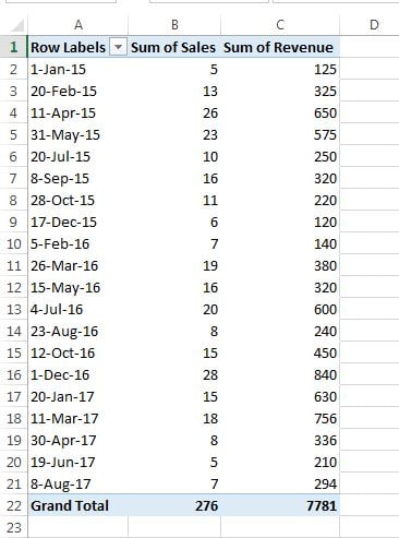
Start from a date-wise pivot table that lists every transaction date down the rows with Sum of Sales and Sum of Revenue beside it.

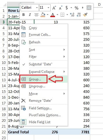
1. Right-click any date in the Row Labels column and click Group. You can also select a date cell and click PivotTable Analyze > Group > Group Field.

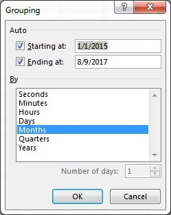
2. The Grouping dialog opens with Seconds, Minutes, Hours, Days, Months, Quarters and Years. Click Months so it is the only highlighted level, check the Starting at and Ending at dates that Excel has read from the data, and click OK.

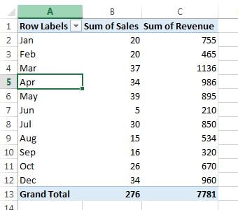
3. The pivot table now shows one row per month with the sales and revenue totals for each.

4. To use more than one level, reopen the dialog and click Years and Quarters so both are highlighted. Excel adds a Years field and a Quarters field and nests them from the largest unit down.

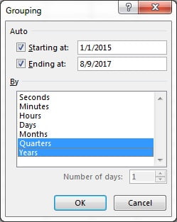
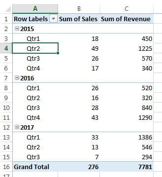
Two details matter here. First, if you pick Months on their own, January of 2024 and January of 2025 are added together, so always add Years when the data spans more than one year. Second, the quarters Excel builds are calendar quarters starting in January. For an April to March fiscal year, group by Months and Years and add a fiscal-quarter column to the source data, or build the quarter in Power Pivot.

How to group dates into weeks

There is no Weeks button, but Days does the job. In the Grouping dialog select Days only, then set Number of days to 7 and change Starting at to the Monday on or before your first date. Excel then labels each bucket with its start and end date. Because Days is exclusive of the other levels, you cannot combine seven-day buckets with Months or Years in the same field; add a WEEKNUM helper column to the source if you need both.

How to group numbers into ranges

Numeric grouping turns a continuous field into a frequency distribution, which is how you answer questions such as how many orders fall between 5,000 and 10,000.

1. Drag the numeric field, for example Revenue, into the Rows area. Put the same field into Values and set it to Count.
2. Right-click any number in the row labels and click Group.
3. Set Starting at to 0, Ending at to a round number above your maximum, and By to the band width, for example 5000. Clear the tick next to Starting at or Ending at to let Excel catch outliers in a single opening or closing band.
4. Click OK. The rows now read 0-4999, 5000-9999 and so on, and the count column is your histogram.

Band widths must be equal. If you need uneven bands such as 0-1000, 1001-10000 and above 10000, build them with a helper column in the source using =IF(A2>10000,"High",IF(A2>1000,"Medium","Low")) and use that column as the row field instead.

How to group text items by hand

Text fields have no dialog. You select the items you want together and group them, which creates a new outer field. Start from a product-wise pivot table showing Product – 1 to Product – 4.

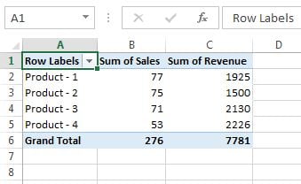
1. Click Product – 1, hold Ctrl and click Product – 2 so both row labels are selected.
2. Right-click the selection and click Group. Excel creates an outer field whose first item is called Group1.

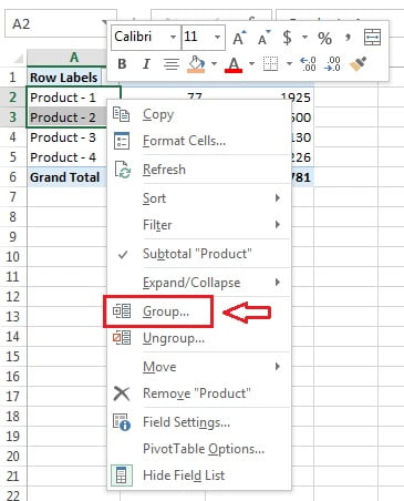
3. Select Product – 3 and Product – 4 and run Group again to create Group2.

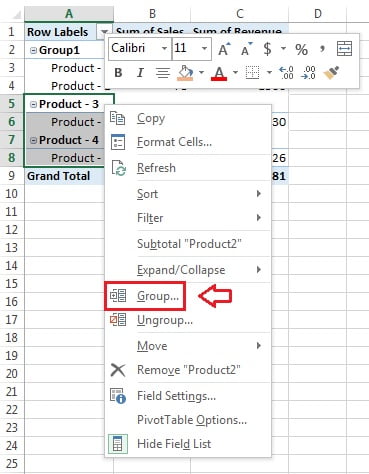
4. Click the Group1 cell and type a real name such as Hardware, then rename Group2 the same way. The new field is listed in the Fields pane as Product2; right-click it and use Field Settings to give it a proper name such as Category.

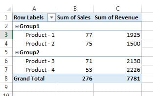
Items you leave out stay on their own at the outer level. Any new product that appears in the source after a refresh is also left ungrouped, so text groups need maintenance. A lookup column in the source data is the durable alternative.

How to ungroup

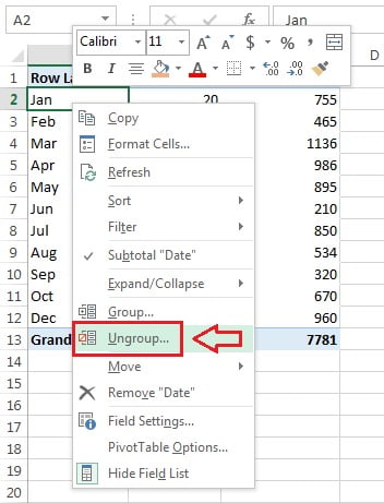
Right-click any grouped item and click Ungroup, or select the field and click PivotTable Analyze > Ungroup. Dates return to individual days and the Years and Quarters fields disappear. To dissolve only one text group, select that group label alone and ungroup it; the other groups survive.

Grouping is shared by every pivot table on the same cache

When you build a second pivot table from the same range and answer Yes to the prompt about sharing data, both reports use one pivot cache. Grouping is a property of that cache, so grouping dates by year in one report instantly regroups the other, and ungrouping does the same damage in reverse. This is the single most common surprise in a multi-sheet report pack.

To keep independent groupings, give the second pivot table its own cache. The reliable way is to copy the source range to a new sheet, or to build the second report from a differently named Table. Refresh, change data source and cache behaviour are covered in the refresh lesson.

Worked example

Suppose the practice file holds these rows.

Date	Product	Revenue
05-Jan-2024	Product – 1	4,200
18-Feb-2024	Product – 3	9,800
02-Feb-2025	Product – 1	6,500
27-Apr-2025	Product – 4	11,300

Put Date in Rows and Revenue in Values, right-click a date, choose Group and select Years and Months. Now drag Years from Rows into Columns. The result is a month down the side, a year across the top, and revenue in the body: Feb shows 9,800 under 2024 and 6,500 under 2025, so the year-on-year movement is visible at a glance. Grouping by Months only would have merged those two figures into one 16,300 cell.

Errors and how to fix them

Message or symptom	Cause	Fix
Cannot group that selection	The date or number column contains text, blanks or errors, so Excel treats the whole field as text	Select the column, use Data > Text to Columns > Finish or add 0 with Paste Special, fill blanks with a real date, then refresh the pivot table
Cannot group that selection on a text field	Only one item was selected, or the selection includes a Grand Total or subtotal row	Select at least two item cells and nothing else
Group is greyed out	The pivot table is built on the Data Model and the field is a date column, or the field sits in the Filters area	Move the field to Rows, or add a proper date table to the model
Dates show as one long list after a refresh	New rows fall outside the range in Starting at and Ending at	Ungroup and group again so Excel reads the new limits
Grouping changed in another sheet	Both pivot tables share one pivot cache	Rebuild the second report from its own copy of the data

Tips and common mistakes

• Check the field type first. If the dates are left-aligned in the source they are text. Convert them before you build the report, not after.
• Add Years whenever the data spans years. Months on their own silently merge the same month from different years.
• Rename generated fields. Years, Quarters and Product2 are Excel names. Field Settings lets you call them Year, Quarter and Category.
• Collapse instead of ungrouping. The minus buttons and Collapse Entire Field hide detail without destroying the grouping.
• Number bands must be equal width. Use a helper column for uneven bands.
• Filter, do not group, for ad hoc periods. A timeline slicer gives a movable date window without changing the cache.
• Blank source rows are the usual culprit. Base the pivot table on an Excel Table so the range never picks up empty rows.

Practice exercise

1. Open the practice file and build a pivot table with Date in Rows and Revenue in Values.
2. Group the dates by Years and Quarters, then move Years to Columns to make a year-on-year quarterly report.
3. Ungroup, then regroup by Days with Number of days set to 7 and a Monday start date, and note how the labels change.
4. Build a second pivot table with Revenue in Rows and Count of Revenue in Values, and group the revenue into bands of 5,000.
5. Type the word test into one date cell in the source, refresh, and try to group. Read the error, undo the change, refresh again and confirm grouping works.

Key takeaways

• Right-click and Group opens the Grouping dialog for dates and numbers; text items are grouped by selecting them first.
• Excel 2016 and later group dates automatically; turn that off in File > Options > Data if you want daily detail.
• Weeks come from Days with Number of days set to 7, not from a Weeks button.
• Cannot group that selection almost always means text, blanks or errors in the field.
• Groups belong to the pivot cache, so every pivot table sharing that cache is regrouped together.
• Grouping never changes the source data and can be undone at any time with Ungroup.

Related lessons

• Pivot Table course hub
• Filters in a pivot table
• Columns in a pivot table for cross-tab reports
• Subtotals and grand totals
• Timeline filter for dates
• Refresh and change data source
• PivotTable Options, settings and troubleshooting
• COUNTIFS function for counting inside date ranges without a pivot table
• Microsoft Support: Group or ungroup data in a PivotTable

Frequently asked questions

How do I group dates by month and year in a pivot table?

Right-click a date in the pivot table, click Group, and in the Grouping dialog click both Months and Years so they are highlighted together, then click OK. Excel adds a Years field above the Months field. Selecting Months alone would add January of every year into a single row, which is rarely what a report needs.

Why does Excel say cannot group that selection?

The field is not consistently a date or a number. One text entry such as N/A, a blank cell, or a date stored as text is enough to break grouping. Select the column in the source, run Data then Text to Columns and click Finish to force conversion, fill any blanks, then refresh the pivot table and try again.

How do I stop Excel grouping dates automatically?

Click File, Options, Data, and tick Disable automatic grouping of Date/Time columns in PivotTables. New pivot tables then show every individual date. Existing reports keep their grouping until you ungroup them. In Excel 2013 and earlier there is no automatic grouping, so the setting does not appear.

Can I group dates by week in a pivot table?

Yes. Open the Grouping dialog, select Days on its own, set Number of days to 7 and set Starting at to the Monday on or before your earliest date. Each row then covers one calendar week. You cannot combine seven-day buckets with Months or Years, so add a WEEKNUM column to the source if you need both levels.

Why did grouping in one pivot table change another one?

Both reports share the same pivot cache, and a group is stored in the cache rather than in the report. Any group, ungroup or date level you apply appears in every pivot table built on that cache. To keep them independent, build the second pivot table from a separate copy of the data or from a differently named Excel Table.

Want the finished version? Ready-made Excel dashboards, trackers and VBA systems are available at NextGenTemplates.com.