Part of the free Module 10: Pivot Tables · Lesson 12 of 20 · Full Excel course
Updated on 5 September 2026 · Works in Excel 365, 2021, 2019 and 2016 unless noted.
To refresh a pivot table in Excel, click inside it and press Alt+F5, or use PivotTable Analyze > Refresh. To update every report and connection in the workbook, press Ctrl+Alt+F5 or click Data > Refresh All. A refresh reads the existing range again; when rows fall outside that range you must also change the data source.
Why a pivot table does not update by itself
When you build a pivot table, Excel copies the source range into a hidden store called the pivot cache and draws the report from that copy, not from the worksheet. This is what makes pivot tables fast on large data, and it is also why editing a cell changes nothing on screen. The report stays frozen until you refresh, which tells Excel to reload the cache from the source and redraw every report that uses it.
Adding rows is a second, separate problem. The cache remembers the exact address you selected at creation, for example Sheet1 A1 to F501. Rows pasted at row 502 sit outside that address, so a refresh reloads the same 500 rows and the totals never move. Fixing that needs a new data source, or better, a source that grows on its own.
Refresh, Refresh All and the shortcuts
Excel gives you two scopes. Refresh touches the selected report and everything that shares its cache; Refresh All touches every pivot table, query and connection in the file. On a workbook with a slow database query, the difference matters.
| Command | Shortcut | Where to find it | What it updates |
|---|---|---|---|
| Refresh | Alt+F5 | PivotTable Analyze > Data > Refresh, or right-click the report | The selected pivot table and any report sharing its cache |
| Refresh All | Ctrl+Alt+F5 | PivotTable Analyze > Refresh > Refresh All, or Data > Queries & Connections > Refresh All | Every pivot cache, Power Query load and external connection in the workbook |
| Refresh Status | none | PivotTable Analyze > Refresh drop-down | Shows progress of a long background refresh |
| Cancel Refresh | none | PivotTable Analyze > Refresh drop-down | Stops a query that is taking too long |
How to refresh a pivot table
- Click anywhere inside the pivot table.
- On the PivotTable Analyze tab (named Analyze in Excel 2016 and 2019) click Refresh in the Data group. Right-clicking the report and choosing Refresh does the same thing, as does Alt+F5.
- To bring the whole workbook up to date, open the Refresh drop-down and choose Refresh All, or press Ctrl+Alt+F5. The same button lives on the Data tab, where it also refreshes Power Query tables and pivot tables at once.
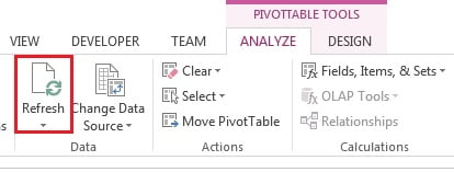
The report redraws at once. New items in the source, such as a new supervisor, appear as new rows; items that no longer exist disappear, unless the field is holding on to them (see the tips below).
What a refresh updates and what it does not
Knowing where the line falls saves a lot of guessing when a report looks wrong.
| Change in the workbook | Does a refresh pick it up? |
|---|---|
| Edited values inside the existing range | Yes |
| New rows inside a Table, or inside a named dynamic range | Yes |
| New rows below a fixed range such as A1:F501 | No, change the data source |
| A new column added to the source | Yes if the column is inside the source range or Table; it appears in the field list, but you still have to drag it into an area |
| A renamed source column | Yes, but the field is dropped from the layout and must be added again |
| Number formats, styles and conditional formatting you applied to the report | Kept, formatting is not reset |
| Date or number grouping you created | Kept, as long as the field still holds the same data type |
| Calculated fields and calculated items | Kept and recalculated |
| Slicer and timeline selections | Kept, so new periods can stay hidden until you widen the selection |
| Column widths | Reset, unless you untick Autofit column widths on update |
How to change the data source of a pivot table
- Click anywhere inside the pivot table.
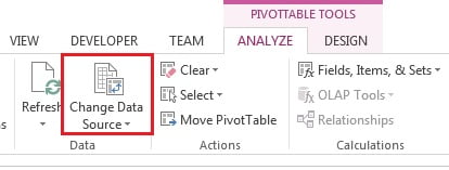
- On the PivotTable Analyze tab click Change Data Source in the Data group, then Change Data Source… in the drop-down.
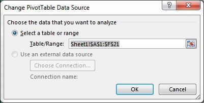
- Excel jumps to the source sheet and opens the Change PivotTable Data Source dialog with the current address in the Table/Range box.
- Select the new range with the mouse, or type it, and make sure the header row is included. A Table name such as SalesData is also accepted here.
- Click OK. The pivot table refreshes itself with the new range.
Use a Table so you never change the source again
The professional habit is to stop resizing ranges altogether. Select any cell in the raw data, press Ctrl+T, confirm that My table has headers is ticked and click OK. Rename the Table on the Table Design tab, for example to SalesData, then build the pivot table from that name. A Table expands automatically when you type or paste under the last row, so the pivot cache always sees the full data set and a plain refresh is enough forever. Building the report this way is covered in Insert a Pivot Table in Excel.
To move an existing report onto a Table, convert the source with Ctrl+T, then open Change Data Source and replace the address with the Table name. You only ever do this once.
Make the refresh automatic
Refresh when the file opens
- Right-click the pivot table and choose PivotTable Options.
- Open the Data tab.
- Tick Refresh data when opening the file and click OK.
Everyone who opens the workbook now sees current figures. The same tab holds Number of items to retain per field, the setting that clears stale filter entries. More of these switches are explained in PivotTable Options, Settings and Troubleshooting.
Refresh with a short VBA macro
Two snippets cover almost every request. Put the first in a standard module and run it from a button; put the second in the code window of the sheet that holds the raw data so the report follows every edit. Save the file as .xlsm.
' Standard module: refresh every pivot table and query
Sub RefreshEverything()
    ThisWorkbook.RefreshAll
End Sub

' Sheet module of the data sheet: refresh after any edit in columns A to F
Private Sub Worksheet_Change(ByVal Target As Range)
    If Intersect(Target, Me.Range("A:F")) Is Nothing Then Exit Sub
    Application.EnableEvents = False
    ThisWorkbook.RefreshAll
    Application.EnableEvents = True
End Sub
Turning events off while the refresh runs stops the macro triggering itself. If you want one report only, use Sheets("Report").PivotTables(1).RefreshTable instead of RefreshAll. New to macros? Start with the Excel VBA course.
External data and Power Query
When the source is a Power Query load, a database, a text file or the Data Model, the connection sits beside the pivot cache and Refresh All updates both in one click, query first, then the report. For scheduled updates, open Data > Queries & Connections, right-click the connection, choose Properties and tick Refresh every N minutes or Refresh data when opening the file. Reports built on the Data Model, such as the distinct count in Pivot Table from Multiple Sheets, behave the same way.
Worked example
Open the practice file Pivot-Table.xlsx and build a pivot table with Supervisor in Rows and Revenue in Values. Now add three rows at the bottom of the source for a new supervisor, Nadia, worth 12,000 in total, and press Alt+F5.
| Supervisor | Before | After refresh only | After extending the source |
|---|---|---|---|
| Alex | 184,300 | 184,300 | 184,300 |
| Priya | 151,900 | 151,900 | 151,900 |
| Nadia | not present | still not present | 12,000 |
| Grand Total | 336,200 | 336,200 | 348,200 |
The middle column proves the point: the refresh worked, but the range did not include the new rows. Open Change Data Source, extend the address by three rows and click OK to get the last column. Then undo everything, press Ctrl+T on the source, point the report at the Table name and add the three rows again. This time Alt+F5 alone gives you 348,200.
Tips and common mistakes
- Old items still listed in filters and slicers. PivotTable Options > Data > Number of items to retain per field set to None, then refresh, clears deleted names.
- Column widths jump on every refresh. Untick Autofit column widths on update on the Layout & Format tab of PivotTable Options.
- One cache, one refresh. Reports built from the same range with Insert > PivotTable share a pivot cache, so refreshing one refreshes all of them and a grouping made in one appears in the others.
- Copying a sheet copies the cache link. The duplicated report still points at the original source, so check Change Data Source after copying a sheet into a new file.
- New column, empty layout. A column added to the source appears in the field list after the refresh but Excel never places it for you; drag it into Rows, Columns or Values yourself.
- File size grows. Untick Save source data with file on the Data tab and tick refresh on open, and the cache is rebuilt instead of stored.
- Blank headers break everything. Every column in the source range needs a header before a refresh or a source change will work.
Errors and how to fix them
| Message | Cause | Fix |
|---|---|---|
| Reference isn’t valid | The source sheet or workbook was renamed, moved or closed, or the range was deleted | Open Change Data Source and point the report at the current sheet name or Table |
| Data source reference is not valid | The file name contains square brackets, or the file is opened from a temporary internet folder | Rename the file without brackets and save it to a normal folder before opening |
| A PivotTable report cannot overlap another PivotTable report | The refreshed report grew into the cells of a second report | Move one report, or leave several blank rows and columns between them |
| The PivotTable field name is not valid | A header cell in the source range is blank | Fill every header, then refresh |
| Deleted names still in the filter list | Excel retains old items per field | Set Number of items to retain per field to None and refresh |
| New rows ignored after a refresh | The rows are outside the fixed source range | Extend the range, or convert the source to a Table with Ctrl+T |
| Refresh is greyed out | The sheet is protected, or the workbook is open read only or shared | Unprotect the sheet and reopen the file with write access |
Practice exercise
- Change one revenue figure in the practice data, press Alt+F5 and watch the total move.
- Add ten rows for a new supervisor below the source, refresh, and confirm nothing happens.
- Use Change Data Source to include the new rows and check the supervisor now appears.
- Convert the source with Ctrl+T, repoint the report at the Table name, add five more rows and prove that a plain refresh is enough.
- Tick Refresh data when opening the file, save, close and reopen the workbook to see the report rebuild itself.
Key takeaways
- Alt+F5 refreshes one pivot table; Ctrl+Alt+F5 or Data > Refresh All updates every report and connection.
- A refresh reloads the existing range only, so new rows outside it need Change Data Source.
- An Excel Table created with Ctrl+T grows on its own and makes Change Data Source unnecessary.
- Refresh keeps your formatting, grouping and calculated fields, but resets column widths unless you turn autofit off.
- PivotTable Options > Data holds refresh on open and the retained items setting that clears stale filter entries.
- ThisWorkbook.RefreshAll in a macro, or a Worksheet_Change event, automates the whole job.
Related lessons
- Pivot Table course: all 20 lessons
- Insert a pivot table in Excel
- PivotTable Options, settings and troubleshooting
- Pivot table from multiple sheets with the Data Model
- Calculated fields and calculated items
- Excel VBA course: write your own refresh macro
- Excel Dashboard course
- Microsoft Support: Refresh PivotTable data
Frequently asked questions
What is the shortcut to refresh a pivot table in Excel?
Alt+F5 refreshes the pivot table you are standing in and every report that shares its cache. Ctrl+Alt+F5 refreshes the whole workbook, including Power Query loads and database connections, and is the same as clicking Data > Refresh All. Both shortcuts work in Excel 2016, 2019, 2021 and 365.
Why does my pivot table not show new data after refreshing?
The new rows sit outside the range the report was built on, so the cache reloads the same block of cells. Use PivotTable Analyze > Change Data Source to extend the address, including the header row, or convert the source to an Excel Table with Ctrl+T so the range grows by itself.
How do I change the data source of a pivot table?
Click inside the report, then choose PivotTable Analyze > Change Data Source > Change Data Source. Excel opens the source sheet and shows the current address in the Table/Range box. Select the new range or type a Table name, keep the header row, and click OK. The report refreshes as soon as you confirm.
Can a pivot table refresh automatically?
Yes, in three ways. Tick Refresh data when opening the file in PivotTable Options > Data. Add a macro that calls ThisWorkbook.RefreshAll and run it from a button or a Worksheet_Change event. For external data, set Refresh every N minutes in the connection properties under Data > Queries & Connections.
Why do deleted items still appear in my pivot table filter?
Excel keeps a list of items that have been seen for each field, so names removed from the source stay in the filter and slicer lists. Right-click the report, choose PivotTable Options > Data, set Number of items to retain per field to None, click OK and refresh once to clear them.
Want the finished version? Ready-made Excel dashboards, trackers and VBA systems are available at NextGenTemplates.com.