Drop-Down List in Excel: Data Validation List Rule

Part of the free Module 6: Data Validation · Lesson 3 of 14 · Full Excel course

Updated on 5 September 2026 · Works in Excel 365, 2021, 2019 and 2016 unless noted.

A drop-down list in Excel is made with the Data Validation List rule. It puts an arrow in the cell and lets the user pick one value from a fixed set, such as Yes, No and NA, or from a range of cells. Anything not in the list is rejected, so entries stay consistent and formulas, PivotTables and dashboards built on the data keep working.

Table of Contents

What the List rule does and when to use it

List is the most used data validation rule because it solves two problems at once. It makes entry faster, since the user clicks instead of typing, and it standardises the values, so you never end up with “Yes”, “yes” and “Y” in the same column. Use it for status fields, departments, regions, categories, months, priorities and any column that later feeds a COUNTIF, a PivotTable or a chart.

The rule offers three ways to supply the items: type them into the Source box, point at a range of cells, or refer to a named range. This lesson covers all three plus the Ignore blank and In-cell dropdown checkboxes. Dependent lists, lists that grow from an Excel Table and searchable lists each have their own lesson later in the course.

Create a drop-down list from typed values

The typed list is the quickest option for a short, fixed set of items.

Select the cells that should carry the drop-down, for example C2:C50.
Go to Data > Data Tools > Data Validation and click Data Validation (shortcut Alt, A, V, V).

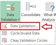
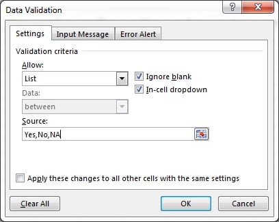
Data Validation button on the Data tab, the starting point for an Excel drop-down list — Data Validation button on the Data tab

On the Settings tab set Allow to List.
In the Source box type the items separated by commas with no spaces: Yes,No,NA.
Leave Ignore blank and In-cell dropdown ticked and click OK.

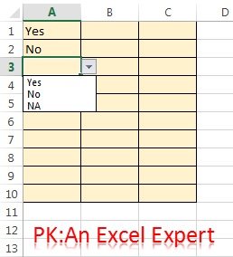
Data Validation dialog with Allow set to List and Yes,No,NA typed in the Source box — List rule with a comma-separated source

Click any validated cell. An arrow appears on its right edge and the drop-down list shows Yes, No and NA. Press Alt+Down Arrow to open the list from the keyboard.

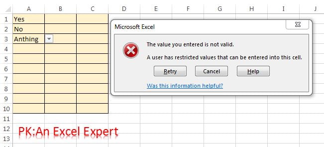
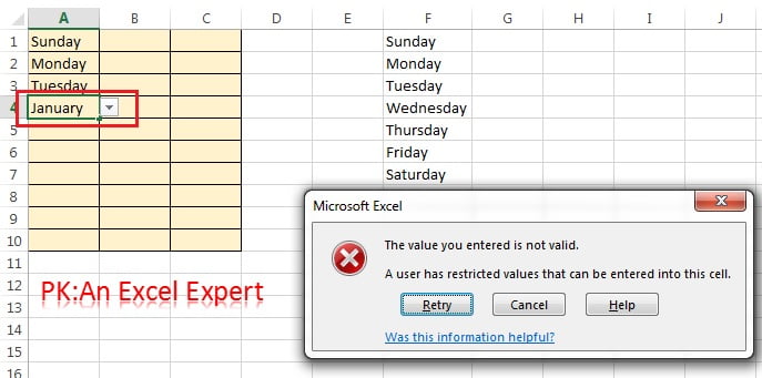
In-cell drop-down list in Excel showing the items Yes, No and NA — The drop-down list in the cell

Type anything else, such as “Maybe”, and Excel rejects it with the default Stop alert.

Excel error message after typing a value that is not in the drop-down list — Error for a value outside the list

The Source box holds at most 255 characters, so typed lists suit three to ten short items. Matching is not case sensitive: “yes” is accepted for “Yes” and stored as typed.

Create a drop-down list from a cell range

For longer lists, or lists that other people maintain, keep the items in cells and point the Source at them. Editing a cell in the range changes the drop-down immediately.

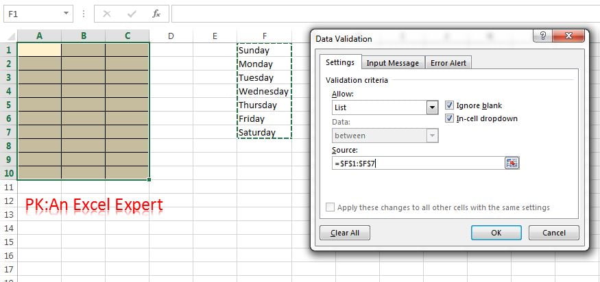
Type the items in a column, here the day names in F1:F7. One item per cell, no blanks, no heading inside the range.
Select the target cells and open Data > Data Validation. Set Allow to List.
Click in the Source box and drag across F1:F7. Excel writes =$F$1:$F$7 with absolute references, which is what you want.
Click OK.

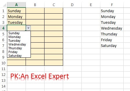
Data Validation Source box referencing the cell range F1:F7 that holds the drop-down list items — Source set to the range F1:F7

The drop-down now lists the seven days in the order they appear in the sheet.

Excel drop-down list of day names sourced from the cell range F1:F7 — Drop-down list sourced from a range

Excel error alert when a value outside the range-based drop-down list is entered — Error for a value outside the range list

The range can sit on another worksheet. Either select it while the dialog is open, which writes =Lists!$A$2:$A$8, or define a name first (Formulas > Define Name) and type =Days in the Source box. A named range is easier to read, reusable on several sheets and does not break if you move the list.

Typed list, cell range or named range: which to use

Source type	What you type in Source	Strengths	Limits	Use it when
Typed list	`Yes,No,NA`	Fastest to set up, no helper cells needed	255-character limit, edits mean reopening the dialog on every validated range	Three to ten fixed items that never change
Cell range	`=$F$1:$F$7` or `=Lists!$A$2:$A$8`	Items are visible and editable in the sheet; changes show at once	Fixed size, so new rows below the range are not picked up; blanks appear as empty items	Longer lists maintained by the sheet owner
Named range	`=Days`	Readable, reusable across sheets, survives moving the list, can point at a Table column	Needs one extra step in Name Manager; a misspelt name gives an error	Lists shared by several columns or sheets, and any list that will grow

Ignore blank and In-cell dropdown explained

In-cell dropdown controls the arrow. Leave it ticked. If you untick it, the cell still rejects values outside the list, but users get no arrow and must type the exact item, which is only useful for silent enforcement behind a form.

Ignore blank decides whether an empty entry is accepted. Ticked (the default), a user can leave the cell empty. Unticked, pressing Enter on an empty cell in edit mode is rejected, although clearing with Delete is still allowed, so it does not make the field mandatory. One side effect matters: when Ignore blank is ticked and the Source is a named range that resolves to a blank cell, Excel accepts any value at all. Keep list ranges free of blank cells and the rule behaves as expected.

When you edit an existing rule, tick Apply these changes to all other cells with the same settings to update every cell that shares it in one go.

Worked example: an order status column

You track orders in A2:D30 and want column D to hold only valid statuses so a summary can count them.

Cell	Value
H1	Status (heading, kept outside the list)
H2	New
H3	Packed
H4	Shipped
H5	Delivered
H6	Cancelled

Select H2:H6, click in the Name Box, type StatusList and press Enter.
Select D2:D30, open Data > Data Validation, set Allow to List and type =StatusList in Source. Click OK.
In J2 enter =COUNTIF($D$2:$D$30,H2) and fill down to J6.

Result: every cell in D2:D30 offers the five statuses, “Shiped” is refused, and J2:J6 shows a correct count per status because no variant spellings can exist. If you later add “Returned” in H7, edit the name to H2:H7 in Formulas > Name Manager and every drop-down updates.

Tips and common mistakes

Use the right separator. Excel uses your Windows list separator. On many European and Indian regional settings it is a semicolon, so Yes;No;NA is needed and a comma list appears as one item.
Keep the heading out of the range. Start the Source at the first item, or “Status” shows up as a selectable value.
Sort the source list. Excel shows items in sheet order, so sort the range once and the drop-down is easy to scan.
Do not paste over validated cells. Pasting a cell replaces the validation as well as the value. Use Paste Special > Values, or see the lesson on copying and removing validation.
Refer to Table columns through INDIRECT. The Source box does not accept a structured reference such as =Table1[Day] directly; use =INDIRECT("Table1[Day]") or a named range that points at the column.
Excel 365 users get AutoComplete. Typing the first letters filters the list. In 2016 to 2021 the list is not filtered, so long lists need the searchable-list technique.

Errors and how to fix them

Symptom	Cause	Fix
“The Source currently evaluates to an error”	Named range misspelt, deleted or pointing at a removed sheet	Check the name in Formulas > Name Manager and retype it in Source
Whole list appears as one item, “Yes,No,NA”	Regional list separator is a semicolon	Separate items with `;`, or move the items to cells and reference the range
No arrow on the cell	In-cell dropdown unticked, or the cell is not active	Open the rule and tick In-cell dropdown; the arrow only shows on the selected cell
Drop-down shows empty items	Blank cells inside the source range	Remove the blanks or shorten the range; use a Table-based list if it must grow
“This value doesn’t match the data validation restrictions”	Entry is not an exact item, for example an extra space	Pick from the list, or change the Error Alert style if free entry is acceptable
Validation vanished after a paste	Copy and paste overwrote the rule	Reapply the rule, then paste values only in future

Practice exercise

In a blank sheet add a typed drop-down with Low,Medium,High to B2:B20 and test that “Urgent” is rejected.
List twelve month names in a column on a second sheet named Lists. Create a drop-down in C2:C20 that references them across sheets.
Name the month range Months and change the rule in C2:C20 to =Months. Confirm it still works.
Untick In-cell dropdown on one cell, note what changes, then tick it again.
Add a COUNTIF summary that counts each priority from B2:B20.

Key takeaways

The List rule under Data > Data Validation creates the standard Excel drop-down list.
Type short fixed lists straight into Source; keep longer lists in cells and reference the range or a named range.
Keep In-cell dropdown ticked so users see the arrow; Ignore blank only controls empty entries and misbehaves with blank source cells.
Matching is exact but not case sensitive, and the 255-character limit applies only to typed lists.
Dependent lists, Table-based dynamic lists and searchable lists build on this rule and have their own lessons.

Related lessons

Frequently asked questions

How do I create a drop-down list in Excel from another sheet?

Type the items on the second sheet, open Data > Data Validation on the target cells, set Allow to List, click in Source and switch to the other sheet to select the range. Excel writes a reference such as =Lists!$A$2:$A$8. Naming the range first and typing =Months is cleaner and works in every version from 2010 onwards.

Why does my drop-down show all items as one entry with commas?

Your Windows regional settings use a semicolon as the list separator, so Excel treats Yes,No,NA as a single item. Separate the items with semicolons instead, or put them in cells and reference the range, which works regardless of locale and is easier to maintain.

How many items can an Excel drop-down list hold?

A typed list is limited by the 255-character Source box, roughly 20 to 30 short words. A range or named range has no practical limit and can hold thousands of items, but the drop-down shows only eight at a time, so very long lists need Excel 365 AutoComplete or the searchable-list technique covered later in this course.

Can I make the drop-down list font bigger?

No. The in-cell drop-down uses a fixed font size that cannot be formatted. Practical workarounds are raising the sheet zoom while the list is used, or replacing the validation with a Form Control combo box from the Developer tab, which has adjustable size and can be linked to a cell.

How do I remove a drop-down list from a cell?

Select the cells, open Data > Data Validation and click Clear All, then OK. To find every validated cell on a sheet first, press F5, click Special and choose Data validation. The lesson on copying, finding and removing validation covers this in detail.

Video lessons: watch the free Excel tutorials on PK: An Excel Expert on YouTube.

Want the finished version? Ready-made Excel dashboards, trackers and VBA systems are available at NextGenTemplates.com.