Top-Bottom preset is used to highlight the Top n or Bottom n items in the excel cell range. By using this preset we can highlight Top or bottom performers in our data.
How to use Top/Bottom Rules
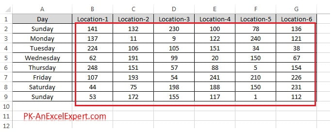
Let’s say we have day wise/ location wise sales data as given in below image and we have to highlight the Top 10 numbers of sales.
- Select the Range “B2:G9”
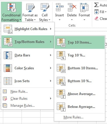
- Goto Home tab>>Conditional Formatting>>Top/Bottam Rules>>Top 10 Items
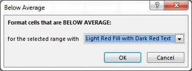
- Below given window will be opened
- By default number is 10, however you can take another number in place of 10.
- Choose a format form the list. By default it is “Light Red Fill with Dark Red Text“
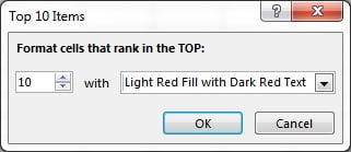
- Click on OK button
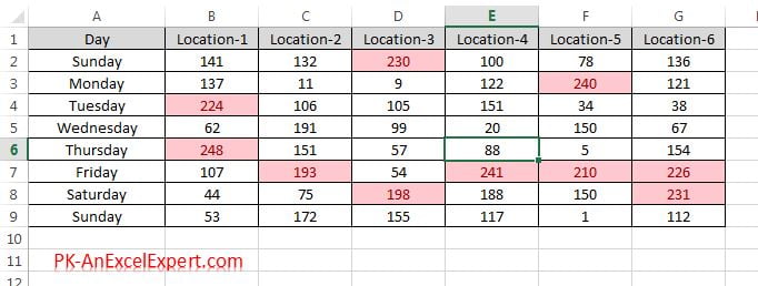
- Formatting will be applied on Top 10 numbers
Below are the other option available in Top/Bottom Rules
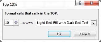
- Top 10 % : Top 10% items can be highlighted by using this option.
Example: if we have 50 Items then it will highlight 5 Top items. If we have 49 Items then it will highlight top 4 items only.If two top items have same numbers then, it will highlight 6 number.
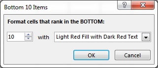
- Bottom 10 Items: Bottom 10 items can be highlighted by using this option.
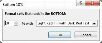
- Bottom 10 % : Bottom 10% items can be highlighted by using this option.
Example: if we have 50 Items then it will highlight 5 bottom items. If we have 49 Items then it will highlight bottom 4 items only.If two bottom items have same numbers then, it will highlight 6 number.
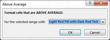
- Above Average : Numbers which are above the average of entire range, can be highlighted by using this option.
Example: If we have average of 50 number 130 then it will highlight all the number which are greater than 130.
- Below Average: Numbers which are blow the average of entire range, can be highlighted by using this option.
Example: If we have average of 50 number 130 then it will highlight all the number which are less than 130.
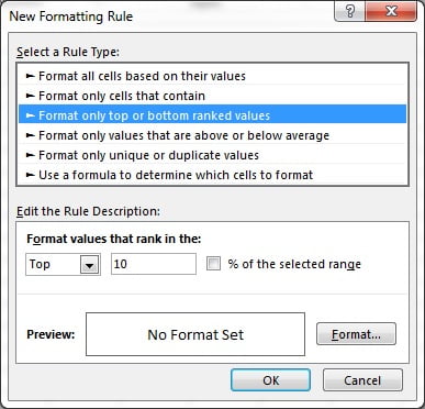
- More Rules: If you click on More Rules option then below given window will be opened. We will learn this in upcoming chapters.
![]()
![]()