Part of the free Module 7: Conditional Formatting · Lesson 1 of 15 · Full Excel course
Updated on 5 September 2026 · Works in Excel 365, 2021, 2019 and 2016 unless noted.
Highlight Cells Rules are the seven preset conditional formatting rules in Excel that colour a cell when its value passes a simple test: Greater Than, Less Than, Between, Equal To, Text that Contains, A Date Occurring and Duplicate Values. You find them under Home > Conditional Formatting > Highlight Cells Rules, and each one needs only a value and a format to work.
What Highlight Cells Rules do
A Highlight Cells Rule compares every cell in the selected range with a value you type, or a cell you point to, and applies a fill, font colour or border when the comparison is true. The format is live. Change the number in the cell and the highlight appears or disappears on the next recalculation, so the rule keeps working long after you set it up.
Use these presets when you need a quick visual check on a range: sales below target, invoice numbers entered twice, deliveries due this week, or every row that mentions a particular customer. They are the fastest way into conditional formatting because the dialog is tiny and the defaults are sensible. When you need something the presets cannot express, such as “greater than or equal to” or “blank cells”, the same menu offers More Rules, which opens the full New Formatting Rule dialog covered later in this course.
The seven presets compared
| Preset | Highlights cells that | What you enter | Typical use |
|---|---|---|---|
| Greater Than | Are larger than the value | One number, date or cell reference | Sales above target |
| Less Than | Are smaller than the value | One number, date or cell reference | Stock below reorder level |
| Between | Fall inside two limits, both limits included | Lower and upper value | Scores in a pass band |
| Equal To | Match the value exactly (text is not case-sensitive) | One number or text | Status equal to “Pending” |
| Text that Contains | Contain the characters anywhere in the cell | Text fragment | Product names containing “Pro” |
| A Date Occurring | Hold a real date inside a relative period | Pick from a list (Yesterday to Next month) | Tasks due this week |
| Duplicate Values | Appear more than once in the selection (or only once, if you choose Unique) | Duplicate or Unique | Repeated invoice numbers |
Every preset shares the same dialog layout: a criteria box on the left and a with drop-down on the right that holds the format choices.
Step by step: highlight values greater than 184
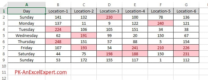
The example uses a day-wise, location-wise sales table in the range B2:G9. The same steps apply to every preset; only the criteria box changes.
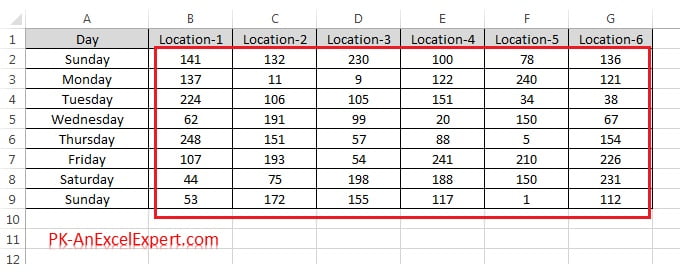
- Select the data range B2:G9. Select only the numbers, not the header row or the day labels.
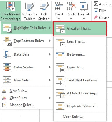
- Go to Home > Conditional Formatting > Highlight Cells Rules > Greater Than.
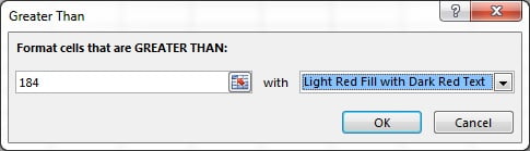
- In the Greater Than dialog, type 184 in the value box. You can also click a cell, which enters a reference such as
=$I$1, so the threshold updates whenever that cell changes.
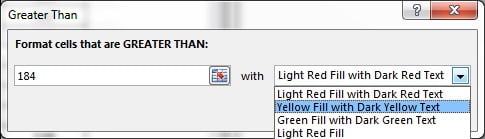
- Open the with drop-down and pick a format. The six presets are Light Red Fill with Dark Red Text, Yellow Fill with Dark Yellow Text, Green Fill with Dark Green Text, Light Red Fill, Red Text and Red Border. Choose Custom Format to open the Format Cells dialog and set your own number format, font, border and fill.
- Click OK. Every cell greater than 184 is highlighted. Cells equal to 184 are not, because the test is strictly greater than.
Preset formats and Custom Format
The six preset formats cover the usual traffic-light needs: red for problems, yellow for warnings, green for good. They only change fill and font colour, so they never disturb the number format. Custom Format is worth knowing for three reasons. First, it lets you match your company colours. Second, it can apply a number format, so a rule can show negative values in brackets or add a currency symbol only when a condition is met. Third, it can set a border, which is often clearer than a fill on a printed report. One limit applies to every conditional format: you cannot change the font name or font size, only style, colour, underline and strikethrough.
The other Highlight Cells Rules presets
All the presets follow the same three moves: select the range, choose the rule, enter the criteria and pick a format.
Less Than
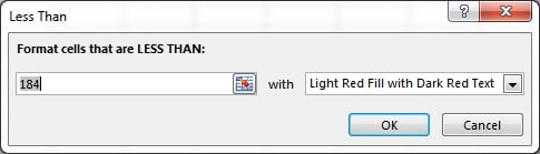
Highlights cells whose value is smaller than the number you enter. It is the natural partner of Greater Than: apply Greater Than in green and Less Than in red to the same range and you have a two-colour target check. For a minimum target of 150, enter 150 and pick Light Red Fill with Dark Red Text.
Between
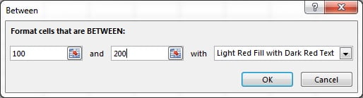
Highlights values that fall inside two limits, and both limits count as inside. Enter the lower value first and the upper value second. If you swap them, Excel still understands the range, but the dialog is easier to read when the order matches the labels. Between accepts dates too, so 01/09/2026 and 30/09/2026 highlights everything dated in September.
Equal To
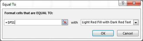
Highlights cells that exactly match a number or a piece of text. Text matching ignores case, so “pending” matches “Pending”, but it must be the whole cell: “Pending review” does not match. Equal To is the right choice for status columns and codes.
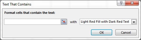
Text that Contains
Highlights cells that contain the characters you type anywhere in the cell, so Loc matches “Location-1” and “Relocation”. Matching ignores case. Use it for product names, comments or status labels where the keyword may sit inside a longer entry. It does not accept wildcards; the fragment itself is the wildcard.
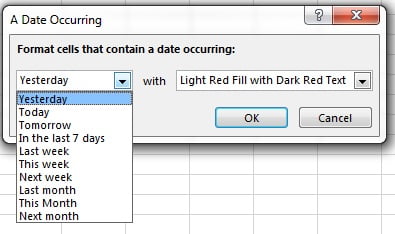
A Date Occurring
Works only on real Excel dates, not on text that looks like a date. The drop-down offers ten relative periods: Yesterday, Today, Tomorrow, In the last 7 days, Last week, This week, Next week, Last month, This month and Next month. The periods follow the system date, so the highlights move forward every day without any edit to the rule. For “overdue” or “due in 3 days” you need a formula rule instead; that is covered in the dates lesson later in the course.
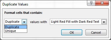
Duplicate Values
Highlights every value that appears more than once in the selection, including the first occurrence. Switch the left drop-down to Unique to highlight the values that appear only once instead. The check is not case-sensitive and treats 100 and “100” stored as text as different values.
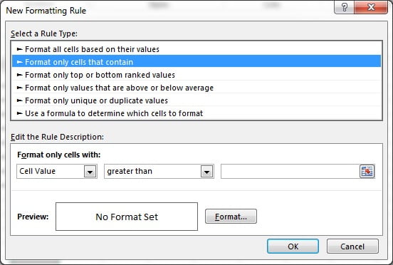
How the presets relate to the New Rule dialog
Every Highlight Cells Rule is a shortcut to one of the rule types in the New Formatting Rule dialog. Greater Than, Less Than, Between and Equal To create a Format only cells that contain rule with Cell Value as the field. Text that Contains creates the same rule type with Specific Text. A Date Occurring uses Dates Occurring, and Duplicate Values maps to Format only unique or duplicate values. Open Manage Rules after applying a preset and click Edit Rule; you will see the full dialog, where you can change the operator to greater than or equal to, add “not between”, or target blanks and errors.
Worked example: target check on a sales table
A manager wants three things on this sales extract: cells above 180 in green, cells below 150 in red, and any duplicate figure flagged for checking. Sample data:
| Day | Location-1 | Location-2 | Location-3 |
|---|---|---|---|
| Monday | 192 | 148 | 176 |
| Tuesday | 165 | 192 | 131 |
| Wednesday | 184 | 171 | 203 |
- Select B2:D4 (the nine numbers).
- Highlight Cells Rules > Greater Than, enter 180, choose Green Fill with Dark Green Text, OK.
- With the same range selected, Highlight Cells Rules > Less Than, enter 150, choose Light Red Fill with Dark Red Text, OK.
- Highlight Cells Rules > Duplicate Values, choose Custom Format, set a bold font and a thick border, OK twice.
Result: 192, 184 and 203 turn green; 148 and 131 turn red; both 192 cells also get the bold border because the value repeats. Wednesday’s 184 stays unformatted by the first rule if you had entered 184 instead of 180, which is why the threshold should sit just below the value you want to catch. To let the manager change the targets, type 180 in cell G1 and 150 in cell G2, then edit each rule’s value box to =$G$1 and =$G$2. The dollar signs lock the reference so every cell in the range compares with the same input cell.
Tips and common mistakes
- Exclude headers from the selection. Text is treated as larger than any number, so a header row lights up in a Greater Than rule.
- Numbers stored as text are ignored. A green triangle in the corner of the cell is the warning sign. Convert with Text to Columns or the VALUE function before applying numeric rules.
- Do not apply the same preset twice. Each application adds a new rule. Check Manage Rules before adding another, or edit the existing one.
- Use a cell reference for thresholds.
=$G$1in the value box means the target can change without opening the rule. - Greater Than excludes the value itself. For “at least 184” use More Rules and choose greater than or equal to.
- Clear rules, do not paint over them. Removing the fill by hand leaves the rule active. Use Home > Conditional Formatting > Clear Rules.
- Dates must be real dates. A Date Occurring and Between ignore text such as “5 Sep 2026” typed with a trailing space.
Practice exercise
Open the course practice file or use any table of numbers, then:
- Highlight every sales figure greater than 184 in green and every figure less than 150 in red.
- Apply a Between rule for 160 to 180 using Custom Format with a blue border only.
- Add a column of dates and use A Date Occurring to mark those falling this month.
- Apply Duplicate Values to the whole table, then switch it to Unique through Manage Rules > Edit Rule.
- Replace the 184 in your Greater Than rule with a reference to an input cell and confirm the highlights change when you type a new target.
Key takeaways
- Highlight Cells Rules are seven presets that format cells that pass a single comparison, and they update live.
- Greater Than, Less Than, Between and Equal To work on numbers and dates; Text that Contains and Equal To work on text.
- A Date Occurring needs real dates and offers ten relative periods that roll forward automatically.
- Duplicate Values can flag either repeated or unique entries.
- Six preset formats plus Custom Format control fill, font colour, border and number format, but never font name or size.
- Every preset is a shortcut into the New Formatting Rule dialog, where More Rules gives you extra operators.
Related lessons
- Conditional Formatting course hub
- Top/Bottom Rules: top 10, bottom 10 percent and above average
- New Rule: Format only cells that contain
- Manage and Clear Rules
- COUNTIF function for counting the cells a rule would highlight
- Microsoft Support: Use conditional formatting to highlight information
Frequently asked questions
Can a Highlight Cells Rule compare with another cell instead of a fixed number?
Yes. Click in the value box and then click the cell that holds the target, or type a reference such as =$I$1. The highlight follows that cell whenever it changes. Keep the dollar signs so every cell in the range compares with the same input cell rather than a shifting relative reference.
Why does Text that Contains highlight nothing on my numbers?
Text that Contains looks at the characters displayed in the cell, while Greater Than, Less Than, Between and Equal To compare the underlying value. A number formatted as currency shows a symbol, but the rule still sees only the number. Use Equal To or Between for numbers and Text that Contains for words and codes.
How do I highlight greater than or equal to a value?
The Greater Than preset is strict. Choose Highlight Cells Rules > More Rules, keep Format only cells that contain, and set the operator to greater than or equal to. Alternatively, apply Greater Than with a threshold one unit lower, for example 183 instead of 184 for whole numbers.
Why does A Date Occurring not highlight my dates?
The dates are probably stored as text. Select the column and look at the alignment: real dates align right by default, text aligns left. Convert them with Data > Text to Columns, choosing Date in the last step, or retype them. The rule also depends on the system date, so check the computer clock if today is wrong.
How do I remove a Highlight Cells Rule?
Select the range and go to Home > Conditional Formatting > Clear Rules > Clear Rules from Selected Cells. To keep some rules and remove one, open Manage Rules, select the rule and click Delete Rule. Clearing the fill colour by hand does not remove the rule, and it will reappear on the next change.
Want the finished version? Ready-made Excel KPI dashboards with target and variance highlighting built in are available at NextGenTemplates.com.