Conditional Formatting Formula in Excel: Highlight Entire Rows

Part of the free Module 7: Conditional Formatting · Lesson 11 of 15 · Full Excel course

Updated on 5 September 2026 · Works in Excel 365, 2021, 2019 and 2016 unless noted.

A conditional formatting formula rule in Excel formats a cell when a logical formula you write returns TRUE. You create it with Home > Styles > Conditional Formatting > New Rule > Use a formula to determine which cells to format. Because you control the formula and the dollar signs, this one rule type can highlight a single cell, an entire row, a whole column or every other row.

How Excel evaluates a formula rule

Excel runs your formula once for every cell in the Applies to range and looks only at the result. TRUE applies the format, FALSE leaves the cell alone. A number counts as TRUE when it is anything other than zero, so =COUNTIF($A:$A,$A2)-1 highlights repeated names without a comparison operator. Text results never format anything, which is why =IF(B2>100,"Yes","No") does nothing at all.

The formula must begin with an equals sign and must be a worksheet formula, not a sentence. Everything Excel can calculate is allowed: comparisons, AND and OR, lookups, date functions, text functions and references to other sheets in the same workbook.

The formula is written for one cell and shifted like a fill

This is the single idea that makes formula rules click. You write the formula as though you were typing it into the active cell of the Applies to range, which is the top-left cell when you drag the selection from top left to bottom right. Excel then copies that formula across the rest of the range exactly as a fill handle would, adjusting every relative part of every reference.

If the Applies to range is A2:G100 with A2 active and the rule is =$D2>100, then cell B2 is tested with =$D2>100, cell A3 with =$D3>100 and cell G57 with =$D57>100. The column stays on D because of the dollar sign; the row moves because it has none. Start the selection anywhere else and the whole grid of results slides, which is the usual reason a rule highlights the wrong rows.

Relative and absolute references in a formula rule

Four reference patterns cover almost every rule you will ever build. Press F4 while the cursor is on a reference to cycle through them.

Reference in the rule	What is locked	What each cell is tested against	Use it for
D2	Nothing	The cell in the same relative position, so each cell tests itself	Highlighting only the cells that fail, such as every even number
$D2	The column	Column D of the cell’s own row	Highlighting the whole row when a value in column D qualifies
D$2	The row	Row 2 of the cell’s own column	Highlighting a whole column when its header or total qualifies
$D$2	Column and row	One fixed cell, the same for every cell in the range	A target, search box, drop-down or checkbox cell that drives the rule

Reading the pattern backwards works too. If the highlight should spread sideways across a row, lock the column. If it should spread downwards through a column, lock the row. If every cell must look at one input cell, lock both.

Press F2 before you use the arrow keys

The formula box in the New Formatting Rule dialog starts in point mode. Pressing an arrow key inserts a cell reference instead of moving the cursor, so an edit quickly turns =$D2>100 into something like =$D2>100A1. Press F2 first to switch the box to edit mode, then the arrow keys move the insertion point normally. Press F2 again if you want to go back to pointing at cells with the mouse or keyboard.

Step by step: your first formula rule

The examples use a day-wise, location-wise sales table in B2:G9, with day names in column A and location headers in row 1.

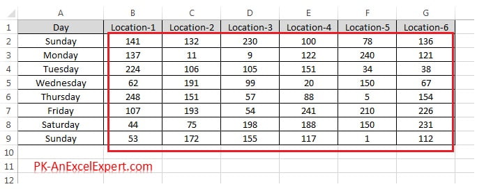
1. Select B2:G9, dragging from B2 so that B2 stays the active cell.
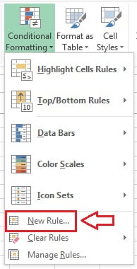
2. Go to Home > Styles > Conditional Formatting > New Rule.

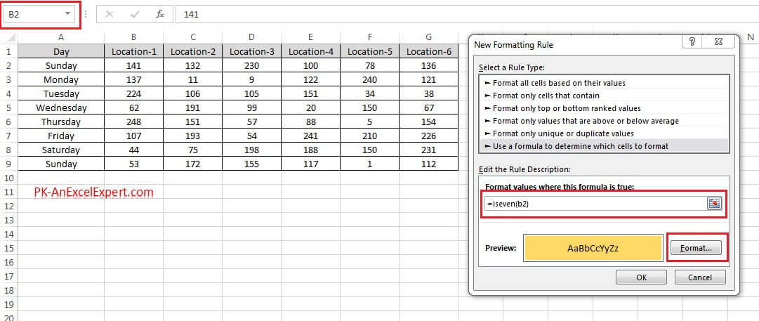
3. In the New Formatting Rule dialog choose Use a formula to determine which cells to format.
4. Type =ISEVEN(B2) in the formula box. B2 is fully relative, so each cell tests its own value.
5. Click Format, pick a fill on the Fill tab and click OK.

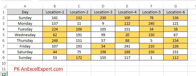
6. Click OK again. Every even value in the range is coloured, and the highlight updates the moment a number changes.

Highlight a whole column

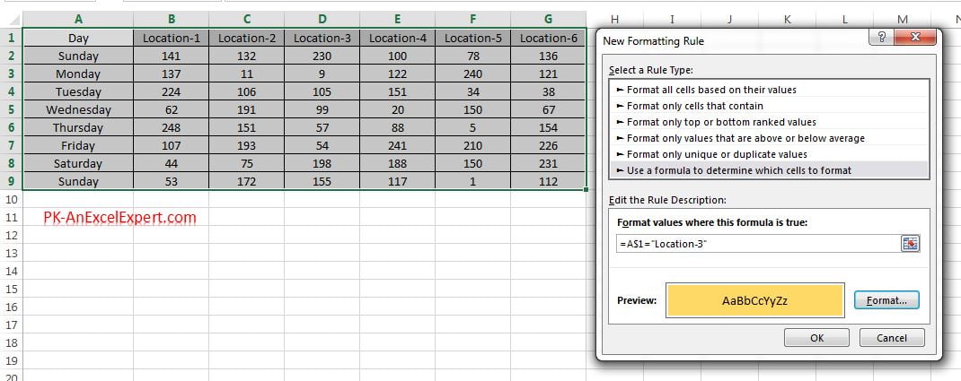
To colour the entire column whose header is Location-3, lock the header row and let the column reference move.

1. Select the whole table including the header row, A1:G9, starting at A1.
2. Create a formula rule with =A$1="Location-3". The dollar sign in front of the row number keeps every test on row 1, so each cell is compared with the header sitting above it.
3. Choose a format and click OK.

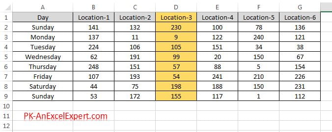
Point the rule at an input cell instead of typed text and the column highlight follows a drop-down: =A$1=$J$1, with a data validation list in J1.

Highlight an entire row

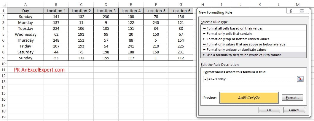
Whole-row highlighting is the most common request in Excel, and it is a locked column away from the rule above.

1. Select the table range A1:G9, starting at A1.
2. Create a formula rule with =$A1="Friday". The dollar sign locks column A, so every cell in a row is compared with that row’s day label.
3. Choose a format and click OK.

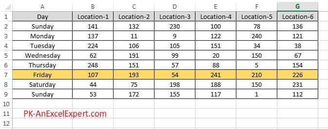
The same pattern works with numbers. On a list where amounts sit in column D and the data starts in row 2, select A2:G200 and use =$D2>100 to colour every row whose amount is over 100. Swap the operator for =$D2<0, =$D2="" or =$D2<>$E2 and the whole row follows.

Shade alternate rows with MOD and ROW

Banded rows are easier to read than plain grids, and a formula rule keeps the bands correct when rows are inserted or deleted, which a manual fill never does.

1. Select the data range, for example A2:G200.
2. Create a formula rule with =MOD(ROW(),2)=0 to shade even-numbered rows, or =MOD(ROW(),2)=1 for odd ones.
3. Choose a light fill and click OK.

ROW returns the row number of the cell being tested and MOD returns the remainder after dividing by 2, so the result alternates all the way down. Use =MOD(COLUMN(),2)=0 for vertical bands, and =MOD(ROW(),4)<2 for bands two rows deep. If the banding should ignore hidden or filtered rows, an Excel Table style is the better tool.

Combine conditions with AND and OR

AND returns TRUE only when every test passes; OR returns TRUE when at least one does. Both accept up to 255 tests, and they nest freely.

Goal	Formula for the rule	What it highlights
Big order from one region	=AND($B2="North",$D2>1000)	Rows where both tests pass
Anything that needs attention	=OR($E2="Overdue",$D2<0)	Rows where either test passes
In a band, but not cancelled	=AND($D2>=500,$D2<=1000,$E2<>"Cancelled")	Rows inside the band with a live status
Missing data	=OR($C2="",$D2="")	Rows with a gap in either column
Weekend dates	=WEEKDAY($A2,2)>5	Rows dated Saturday or Sunday

Multiplication and addition are shorthand for the same logic. =($B2="North")*($D2>1000) behaves like AND because TRUE multiplies as 1, and a plus sign behaves like OR. Stick to AND and OR while you are learning; they read better when someone else opens the file.

Compare two columns

Comparing a plan with an actual is a formula rule in one line. With plan in column C and actual in column D, select the data range starting at C2 and add these rules:

• =$D2<>$C2 to flag any row where the two differ.
• =$D2<$C2 in red for a shortfall, and =$D2>$C2 in green for an overshoot.
• =ABS($D2-$C2)>$H$1 to flag only gaps bigger than the tolerance typed in H1.

To find values in one list that are missing from another, apply =COUNTIF($F:$F,$A2)=0 to column A. The count is zero when the entry does not appear in column F, and zero converts to FALSE, so only the missing entries are highlighted.

Highlight rows containing a piece of text

Equal To matches a whole cell. To catch a fragment inside a longer entry, wrap SEARCH in ISNUMBER:

=ISNUMBER(SEARCH("urgent",$C2))

SEARCH returns the position of the text when it finds it and the error #VALUE! when it does not. ISNUMBER converts that into a clean TRUE or FALSE, which is what the rule needs. SEARCH ignores case and accepts the wildcards ? and *, so “ur?ent” also matches. Use FIND instead of SEARCH when the match must be case-sensitive.

Point the rule at a cell rather than fixed text and you have a live search box: type the keyword in H1, then use =AND($H$1<>"",ISNUMBER(SEARCH($H$1,$C2))). The extra AND stops every row lighting up while the box is empty, because SEARCH finds an empty string in everything.

Why IF is unnecessary

The rule already asks a yes or no question, so the comparison alone is the answer. =B2>100 and =IF(B2>100,TRUE,FALSE) give the same result, and the shorter one is easier to read and quicker to recalculate. IF becomes actively harmful when it returns text: =IF(B2>100,"Yes","No") always returns text, text is not TRUE, and nothing is ever formatted. Keep IF for the rare case where different tests apply in different situations, such as =IF($E2="Closed",$D2>500,$D2>100).

Worked example: a job list with three rules

A small job list in A1:E7, with headers in row 1 and data from row 2:

Job	Owner	Region	Amount	Status
J-101	Asha	North	1250	Open
J-102	Ben	South	90	Urgent review
J-103	Chen	North	640	Open
J-104	Dev	East	1400	Closed
J-105	Eva	North	310	Open
J-106	Farid	South	1180	Urgent review

1. Select A2:E7, dragging from A2 so it is the active cell.
2. Add rule one with =AND($C2="North",$D2>1000) and a green fill. Row J-101 turns green.
3. Add rule two with =ISNUMBER(SEARCH("urgent",$E2)) and a red font. Rows J-102 and J-106 get red text.
4. Add rule three with =MOD(ROW(),2)=0 and a very light grey fill for banding.
5. Open Manage Rules and drag the banding rule to the bottom so the two data rules sit above it.

Result: J-101 is green, J-102 and J-106 carry red text, and the untouched rows keep the grey banding. Because the green rule sets a fill and the red rule sets a font colour, a row that met both conditions would show both. Rules that set the same property do not combine; the one higher in the manager wins.

Debug a formula rule by copying it into a cell

When a rule does nothing, or paints the wrong cells, test the formula on the worksheet.

1. Open Conditional Formatting > Manage Rules, click Edit Rule and copy the formula text.
2. Note the first cell of the Applies to box, for example A2.
3. Type the formula into a spare cell on the same row as that first cell, for example J2, and press Enter. It should show TRUE or FALSE.
4. Fill J2 down beside the data. Every TRUE marks a cell or row the rule will format, so you can see straight away whether the pattern matches what you expected.
5. Fix the dollar signs in the spare column until the TRUEs land correctly, then paste the corrected formula back into the rule and delete the helper column.

Two more checks are worth a minute. Confirm the Applies to range actually covers the data, because copying and filtering can shrink or fragment it. Confirm the rule sits in the right place in the list, since a rule above it may already be applying a conflicting fill.

What a formula rule cannot do

• No other workbooks. A conditional formatting formula cannot reference another workbook, open or closed. Pull the values onto a sheet in the same workbook first, with Power Query or a simple link, then point the rule at that sheet.
• References to other sheets are fine. Excel 2010 and later accept =B2>Targets!$B$1 directly. In Excel 2007 and earlier you needed a defined name.
• No spilled range operator. A dynamic array reference such as =A2# is not accepted in a rule; refer to an ordinary range instead.
• Array behaviour is limited. Simple array logic like =SUMPRODUCT(($A2=$H$2:$H$9)*1)>0 works, but rules are not the place for LAMBDA, LET-heavy formulas or functions that need to spill.
• No volatile functions in big ranges. TODAY, NOW, OFFSET, INDIRECT and RAND recalculate constantly and make a large sheet crawl.
• Font name and size cannot change. Conditional formats control number format, font style and colour, border and fill only.

Tips and common mistakes

• Write the formula for the top-left cell. Select from the top-left corner downwards so the active cell is predictable, or check the Applies to box before you trust the result.
• Do not lock everything. =$B$2>100 tests one cell and then formats the whole range or nothing at all. Lock only the part that must stay fixed.
• Press F2 before editing. Arrow keys insert references into the formula box until you switch to edit mode.
• Never return text. The formula must resolve to TRUE, FALSE or a number. Text and error values format nothing.
• Watch the empty-cell trap. A blank cell counts as zero, so =$D2<100 highlights every empty row. Add a guard: =AND($D2<>"",$D2<100).
• Apply the rule to the data, not the whole sheet. Whole-column ranges such as A:G inflate the file and slow recalculation.
• Check for duplicate rules. Copying rows copies rules, so the manager fills with near-identical entries. Delete the extras and widen the Applies to range of the one you keep.

Errors and how to fix them

Symptom	Cause	Fix
Nothing is highlighted	The formula returns text, or it is missing the leading equals sign	Test the formula in a spare cell and make sure it shows TRUE or FALSE
The whole range is highlighted	An absolute reference such as $B$2 makes every cell give the same answer	Remove the dollar sign from the part that must move
Only the first column is highlighted	The reference is relative when it should lock the column	Change D2 to $D2 for a whole-row highlight
The highlight is one or more rows out	The formula was written for a cell other than the active cell	Rewrite it for the first cell shown in the Applies to box
Excel says the formula is not valid	An arrow key inserted a reference, or a quotation mark is missing	Press F2, clear the box and retype the formula
Blank rows light up	Empty cells evaluate as zero	Add a test such as $D2<>"" inside AND
The rule works, then stops after a paste	Pasting replaced the formats and split the Applies to range	Use Paste Special > Values, then repair the range in Manage Rules

Practice exercise

Open the course practice file or any table of your own, then:

1. Highlight every even number in the data block with =ISEVEN(B2), then change it to =ISODD(B2) and confirm the highlight flips.
2. Colour the whole row for one day of the week with =$A1="Friday", then replace the text with a reference to an input cell so a drop-down controls it.
3. Shade alternate rows with =MOD(ROW(),2)=0, insert a row in the middle and check that the banding repairs itself.
4. Add a two-condition rule with AND, such as amount over 150 and location equal to Location-2, and prove it with a helper column of TRUE and FALSE.
5. Type a keyword in an empty cell and highlight every row containing it using =AND($H$1<>"",ISNUMBER(SEARCH($H$1,$C2))).

Key takeaways

• A formula rule formats a cell whenever the formula returns TRUE, or any non-zero number; text results never format anything.
• Write the formula for the active cell of the Applies to range; Excel shifts it across the range like a fill.
• $D2 highlights whole rows, D$2 highlights whole columns, $D$2 ties every cell to one input cell and D2 tests each cell on its own.
• Press F2 in the formula box before using the arrow keys, or Excel inserts references instead of moving the cursor.
• AND, OR, MOD with ROW, COUNTIF and ISNUMBER with SEARCH cover most real highlighting jobs.
• Test any doubtful rule by pasting its formula into a spare cell beside the data and reading the TRUE and FALSE results.
• Rules cannot reference another workbook, use spilled ranges or change font name and size.

Related lessons

• Conditional Formatting course hub
• Highlight dates: due today, overdue, this week and weekends
• Conditional formatting based on another cell, a drop-down or a checkbox
• Rule precedence and Stop If True
• New Rule: Format only cells that contain
• Manage and clear conditional formatting rules
• AND function and SEARCH function used in the rules above
• Create a drop-down list to drive a formula rule from an input cell
• Microsoft Support: Apply colour to alternate rows or columns
• Microsoft Support: Using IF with AND, OR and NOT

Frequently asked questions

How do I highlight an entire row based on one cell value?

Select the whole data range starting at its top-left cell, choose Use a formula to determine which cells to format, and enter a formula that locks the column of the test cell, such as =$D2>100. The dollar sign keeps every cell in the row looking at column D, while the row number moves down the range, so the format spreads sideways across each qualifying row.

Why does my formula rule highlight the wrong rows?

The formula was written for a cell other than the active cell of the Applies to range. Open Manage Rules, read the first cell in the Applies to box, and rewrite the formula as though you were typing it into that cell. Also check the dollar signs: locking the wrong part shifts the whole pattern of results.

Can I use IF in a conditional formatting formula?

You can, but you almost never need to. The rule already expects a TRUE or FALSE answer, so =B2>100 does the same work as =IF(B2>100,TRUE,FALSE). Avoid an IF that returns text, because text never triggers a format. Reach for IF only when the test itself must change, for example when closed jobs use a different threshold.

Can a conditional formatting formula refer to another sheet or workbook?

Another sheet in the same workbook is fine in Excel 2010 and later, for example =B2>Targets!$B$1. Another workbook is not allowed at all, even when it is open. Copy or link the values you need onto a sheet in the same file, then point the rule at that sheet.

How do I shade every other row in Excel?

Select the data range and add a formula rule with =MOD(ROW(),2)=0 and a light fill. ROW gives the row number and MOD returns the remainder after dividing by 2, so the shading alternates and repairs itself when rows are inserted or deleted. Use =MOD(COLUMN(),2)=0 for vertical bands.

Want the finished version? Ready-made Excel KPI dashboards with row highlighting and variance rules already built in are available at NextGenTemplates.com.