“Format only cells that contain” rule is used on cells number, specific text, dates, blanks, non-blanks, error etc. This use is most commonly used in MS Excel.
To apply “Format only cells that contain” rule below are the steps
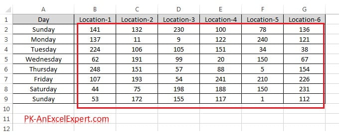
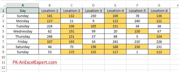
- Select the range on which you want to apply the conditional formatting
- As in below image select “B2:G9”
- Go to Home tab>>Conditional Formatting>>New Rules
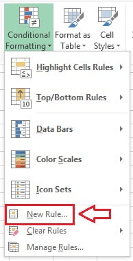
- New formatting rule window will be opened.
- Select “Format only cells that contain window” option.
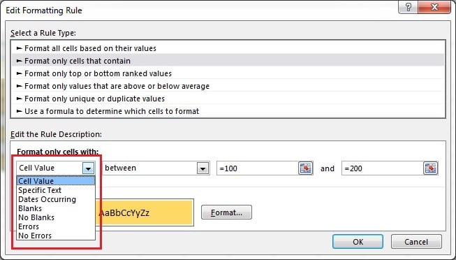
There 7 option available in format only cells with drop down
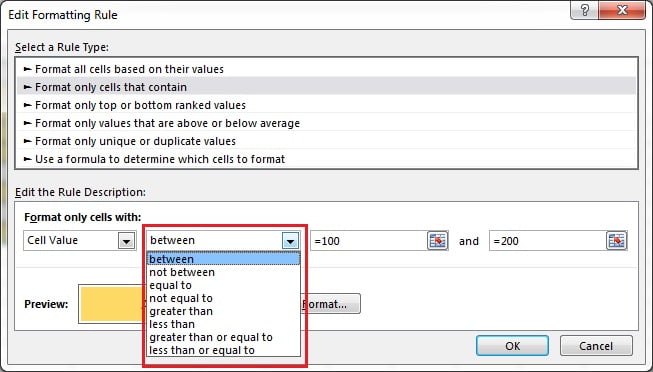
1. Cell Value:
In the cell value option we can put the conditional formatting on the base of value which is available in cells. for exam we want to highlight cells which have the value between 100 and 200.
- Select the Cell Value
- Select the between
- put the minimum number 100 and maximum 200
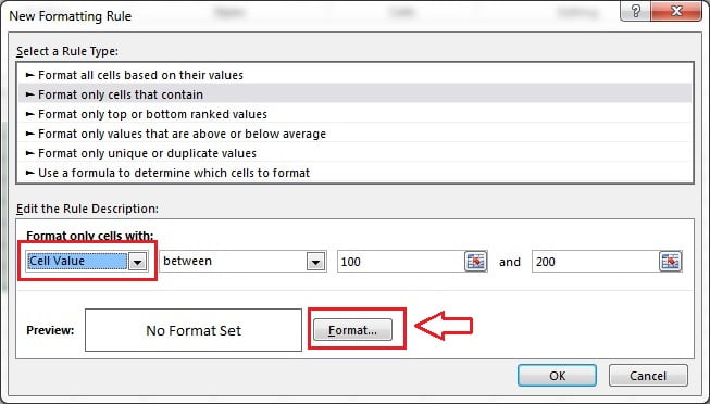
- Click on Format button.
- Format Cells window will be opened.
- You can give any cell background color, Border, font style or font color, and Number format.
- We are taking cell background color only.
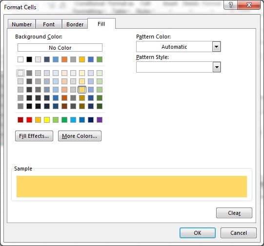
- Click on OK button to apply this conditional formatting.
- Data set with this conditional formatting will look like below image.
In place of between you can use “not between”, “equal to”, “not equal to”, “greater than”, “less than”, “greater than or equal to” and “less than or equal to” in the conditions for cell value
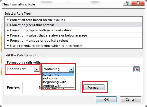
2. Specific Text:
You want to highlight a specific text then you can use this option. for example you want to highlight all the excel cells which containing a specific text.
Available condition for Specific Text are “containing“, “not containing“, “beginning with” , “ending with”
Give the format whatever you want to apply on the excel cells.
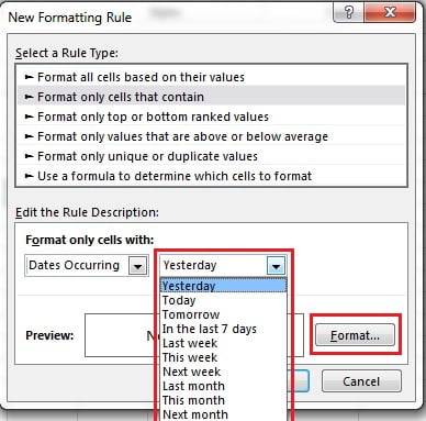
3. Dates Occurring:
You want to highlight a dates for example date of Yesterday then you can use Dates Occurring option.
Available condition for Dates Occurring are “Yesterday“, “Today“, “Tomorrow” , “In the last 7 days“, “Last Week“, “This Week” , “Next Week“, “Last Month“, “This Month” and “Next Month”
Give the format whatever you want to apply on the excel cells.
4. Blanks:
After applying the Blanks rule, all the blanks cells will be highlighted in the selected range. Give the format whatever you want to apply on the excel cells.

5. No Blanks:
After applying the No Blanks rule, all the non blank cells will be highlighted in the selected range. Give the format whatever you want to apply on the excel cells.

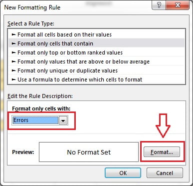
6. Errors:
After applying the Errors rule, all the cells will be highlighted in the selected range which have errors (like -#DIV/0!, #NAME?,#N/A, #VALUE! etc ). Give the format whatever you want to apply on the excel cells.
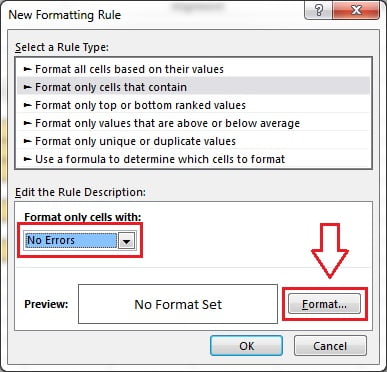
6. No Errors:
After applying the No Errors rule, all the cells will be highlighted in the selected range which do not have any error (like -#DIV/0!, #NAME?,#N/A, #VALUE! etc ). Give the format whatever you want to apply on the excel cells.
![]()
![]()