Sort by Colour in Excel: Cell Colour, Font Colour and Icon Sets

Part of the free Module 4: Sort and Filter · Lesson 2 of 11 · Full Excel course

Updated on 5 September 2026 · Works in Excel 365, 2021, 2019 and 2016 unless noted.

To sort by colour in Excel, open the AutoFilter drop-down on the coloured column, point to Sort by Color and click the swatch you want on top. For more than one colour, use Data > Sort, set Sort On to Cell Color, Font Color or Conditional Formatting Icon, and add one level per colour. Excel groups the chosen colour together and leaves the other rows in their original order.

Why sort by colour is useful

Colour is usually the first thing people add to a worksheet. Yellow means follow up, red text means overdue, green means approved. Sorting by that colour turns informal highlighting into a working list without adding a status column. It works with fills and fonts you applied by hand, and with colours and icons applied by Conditional Formatting rules, so you can sort “cells above target” or “duplicate values” to the top in one step. US readers searching for “sort by color in Excel” are looking for exactly the same feature; only the spelling differs.

One rule to remember before you start: Excel has no built-in idea of which colour comes first. There is no default colour order, so a single-colour sort puts one colour on top and leaves everything else as it was. To rank several colours you must tell Excel the order yourself in the Sort dialog. The sections below cover both cases.

The sample data

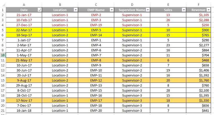
The sales table below has several Date cells highlighted with a yellow background and several Employee names written in red font. You will bring each group to the top in turn. The same table is in the course practice file if you want to follow along.

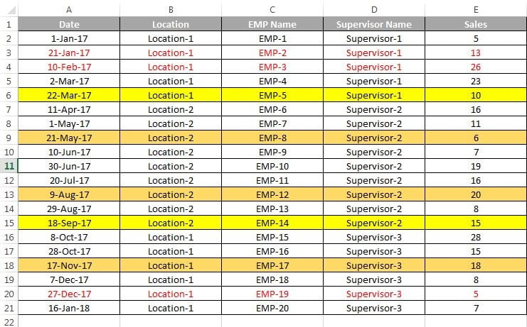
How to sort by cell colour with the filter drop-down

1. Click any cell inside the data and press Ctrl+Shift+L (or choose Data > Sort & Filter > Filter) to add the AutoFilter arrows.
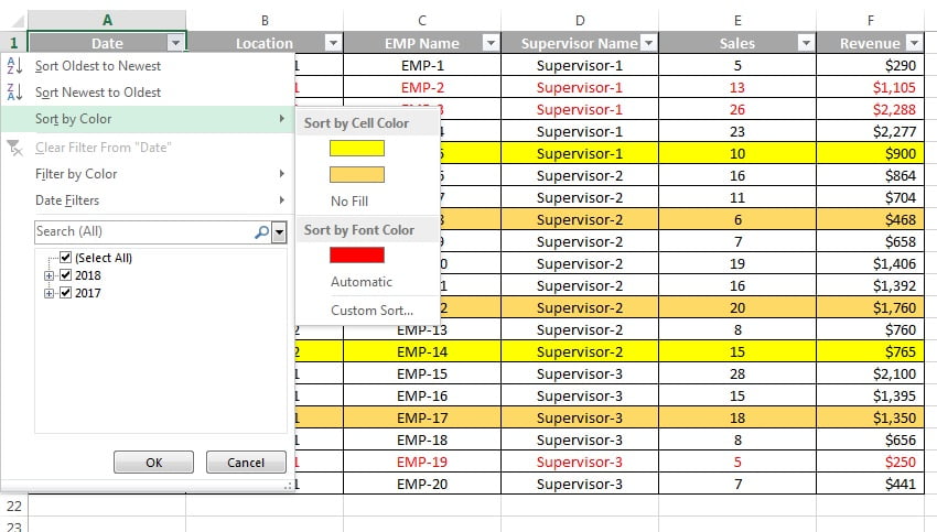
2. Open the drop-down arrow on the Date column, the column that contains the yellow cells.
3. Point to Sort by Color. The submenu lists every fill colour used in that column under Sort by Cell Color.
4. Click the yellow swatch.

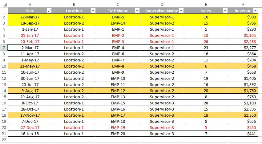
Every row whose Date cell is yellow moves to the top of the table. The remaining rows follow in their original order, because Excel treats “no fill” as a single group and does not reorder it.

How to sort by font colour

1. With the filter arrows still on, open the drop-down on the Employee column, which contains the red text.
2. Point to Sort by Color and look under Sort by Font Color.
3. Click the red swatch.

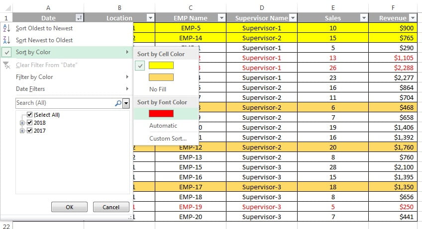
Rows with red employee names are now grouped at the top of the list. The earlier yellow sort is replaced, not combined; the drop-down applies one colour on one column at a time.

The right-click shortcut

You do not need filter arrows at all for a single colour. Right-click any cell that has the fill or font colour you want, point to Sort and choose Put Selected Cell Color On Top or Put Selected Font Color On Top. Excel sorts the whole contiguous range by that column and colour. This is the fastest route when you are reviewing a list and want to gather “all the yellow ones” without touching the ribbon. The same menu also offers Put Selected Cell Icon On Top when the cell carries a conditional formatting icon.

Sort several colours in a chosen order with the Sort dialog

The drop-down and right-click menu handle one colour. To rank red, then yellow, then green, use the Sort dialog and give each colour its own level.

1. Click inside the data and choose Data > Sort & Filter > Sort. Make sure My data has headers is ticked.
2. In Sort by, pick the column that holds the colours.
3. In the Sort On box, choose Cell Color (or Font Color, or Conditional Formatting Icon).
4. In Order, pick the first colour swatch and leave On Top selected.
5. Click Add Level, keep the same column and Sort On setting, and pick the next colour. Repeat for each colour.
6. Optionally add a final value level, for example Sales largest to smallest, so rows are ordered inside each colour group. Click OK.

Choose On Bottom instead of On Top when you want a colour pushed to the end of the list. Levels are applied from the top down, so the first level wins and later levels only break ties.

Method	Where	Colours per sort	Best for
Filter drop-down	Column arrow > Sort by Color	One	Quick review of a filtered list
Right-click menu	Right-click cell > Sort > Put Selected Cell Color On Top	One	Fastest, no filter arrows needed
Sort dialog	Data > Sort, Sort On = Cell Color / Font Color / Icon	Many, in your order	Ranking red, then yellow, then green
Sort dialog with value level	Colour levels plus a Values level	Many plus a value	Colour groups ordered by amount inside

Sort by conditional formatting icon set

Icon sets (traffic lights, arrows, flags) are sortable too. In the Sort dialog set Sort On to Conditional Formatting Icon, then pick an icon in the Order box and choose On Top or On Bottom. Add one level per icon to get a full red, amber, green ranking. Because the icons are driven by the underlying values, this is often the same result as sorting the numbers, but it is useful when the thresholds are percentiles or custom limits that a plain value sort would not reproduce. Colour scales are the exception: Excel cannot sort by a colour scale gradient, so sort by the value column instead.

Worked example

A team lead marks customer accounts during a review. Red fill means “at risk”, yellow means “watch”, and no fill means “healthy”. They want at-risk accounts first, then watch accounts, and healthy ones last, with the biggest balance first inside each group.

Customer	Balance	Fill colour
Acme Ltd	12,400	None
Bright Foods	8,900	Red
Clover Bank	15,200	Yellow
Delta Motors	21,000	Red
Everly Homes	5,300	Yellow

Steps: Data > Sort. Level 1: Sort by Customer, Sort On Cell Color, Order red, On Top. Add Level. Level 2: Customer, Cell Color, yellow, On Top. Add Level. Level 3: Sort by Balance, Sort On Values, Order Largest to Smallest. Click OK.

Result order: Delta Motors (red, 21,000), Bright Foods (red, 8,900), Clover Bank (yellow, 15,200), Everly Homes (yellow, 5,300), Acme Ltd (no fill, 12,400). The colour levels decide the groups and the value level orders the rows within each group.

Tips and common mistakes

• Open the drop-down on the coloured column. The Sort by Color submenu only lists colours that exist in that particular column. If it is empty or greyed out, you are on the wrong column.
• There is no default colour order. Excel does not know that red is more urgent than yellow. Any ranking beyond one colour must be built level by level in the Sort dialog.
• Similar shades are different colours. Two yellows from different palettes appear as two swatches. Use the Fill Color drop-down’s Recent Colors row so the whole team applies the same shade.
• Conditional formatting colours count. Rows coloured by a rule sort like manual fills, so “sort red on top” may really mean “sort below target on top”. Check which rule produced the colour before you trust the result.
• Removing colour does not undo the sort. Clearing fills leaves rows where they are. Add a serial number column before you sort if you may need the original order back, and press Ctrl+Z straight away if you sorted by mistake.
• Select the whole table, or nothing. Selecting a single column before sorting can reorder that column alone and scramble the rows. Click one cell and let Excel detect the range, or select every column.
• Prefer a status column in shared files. Colours are easy to apply inconsistently. A Status column with a drop-down list is more reliable, and you can still colour it with a Conditional Formatting rule.

Errors and how to fix them

Problem	Cause	Fix
Sort by Color is greyed out	No fill or font colour in the column you opened	Open the drop-down on the column that actually holds the colours
Only one colour moves, the rest stay mixed	Single-colour sort from the drop-down	Use Data > Sort and add one level per colour
Rows no longer match across columns	A single column was selected before sorting	Press Ctrl+Z, click one cell in the data and sort again
Cannot sort by colour scale	Excel does not sort by gradient colour scales	Sort by the underlying value column instead
Colour sort ignores some rows	Blank row or column splits the data range	Remove the blank, or select the full range before sorting

Practice exercise

Download the practice workbook Sort-and-Filter.xlsx and complete these tasks on the sales sheet.

1. Fill five Date cells yellow and write three Employee names in red font. Sort each colour to the top using the filter drop-down.
2. Right-click a yellow cell and use Sort > Put Selected Cell Color On Top. Compare the result with task 1.
3. Fill two more Date cells red. Use the Sort dialog to put red first, yellow second, then Sales largest to smallest.
4. Apply a Conditional Formatting rule that colours Sales above 20 green, then sort green on top.
5. Add a three-arrow icon set to the Sales column and sort the down arrows to the bottom using Sort On = Conditional Formatting Icon.

Key takeaways

• The filter drop-down and the right-click menu sort one colour to the top or bottom in two clicks.
• Excel has no default colour order, so multi-colour ranking is built with levels in the Sort dialog.
• Sort On offers Values, Cell Color, Font Color and Conditional Formatting Icon; colour scales cannot be sorted.
• Rows without the chosen colour keep their original relative order.
• Combine colour levels with a value level to order rows inside each colour group.

Related lessons

• Sort and Filter course hub
• Data sorting in Excel: single, multi-level and custom sort
• Filter by colour in Excel
• Excel sort and filter not working: fixes and case-sensitive sort
• Conditional Formatting course
• Highlight duplicates with Conditional Formatting
• Microsoft Support: Sort data in a range or table

Frequently asked questions

Why is Sort by Color greyed out in Excel?

The column whose drop-down you opened contains no fill or font colours. The Sort by Color submenu only lists colours that exist in that column, so open the arrow on the coloured column itself. If the colour comes from a Conditional Formatting colour scale, it cannot be sorted at all; sort by the value column instead.

Can I sort by more than one colour at once?

Yes. Go to Data > Sort, set Sort On to Cell Color, pick the first colour and On Top, then click Add Level and pick the next colour on the same column. Repeat for every colour. Excel applies the levels from top to bottom, so the first colour listed ends up highest.

Does sort by colour work with conditional formatting?

Yes. Fill colours, font colours and icon sets applied by Conditional Formatting rules appear in the Sort by Color menu and in the Sort dialog exactly like manual formatting. Only colour scales are excluded. Remember the colour reflects a rule, so sorting red on top really sorts the rule’s condition on top.

How do I sort by colour without using a filter?

Right-click a cell that has the colour you want, point to Sort and choose Put Selected Cell Color On Top or Put Selected Font Color On Top. Excel sorts the surrounding data range immediately. For several colours, open Data > Sort and add a level per colour; no filter arrows are needed for either method.

Why does Excel not sort colours in rainbow or alphabetical order?

Excel stores colours as RGB values with no meaning attached, so it has no default order such as red before yellow. A colour sort simply groups the chosen colour together and leaves the rest untouched. To impose an order, list the colours as separate levels in the Sort dialog in the sequence you want.

Want the finished version? Ready-made Excel dashboards, trackers and VBA systems are available at NextGenTemplates.com.