Part of the free Module 4: Sort and Filter · Lesson 5 of 11 · Full Excel course
Updated on 5 September 2026 · Works in Excel 365, 2021, 2019 and 2016 unless noted.
To filter by colour in Excel, switch on AutoFilter with Ctrl+Shift+L, open the drop-down on the coloured column, point to Filter by Color and click a swatch under Filter by Cell Color, Filter by Font Color or Filter by Cell Icon. Only rows with that fill, font colour or icon stay visible; everything else is hidden until you clear the filter.
When to filter by colour
Reviewers highlight cells long before they add status columns: a yellow fill for “check this”, red text for “overdue”. Filtering by that colour lets you work through just those rows, copy them to a follow-up sheet or count them with SUBTOTAL, without writing a formula. Unlike sorting by colour, which only moves matching rows to the top, filtering hides the rest, so the view is clean.
Colour filters work with manual formatting and with fills, fonts and icon sets applied by Conditional Formatting, and they combine with value filters on other columns. US readers will see the ribbon spell it “Filter by Color”; the feature is the same in every English edition.
The sample data
The data set from the course practice file has some Date cells filled yellow and some Employee names in red font.
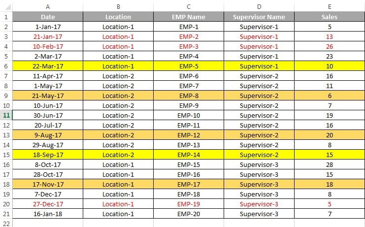
How to filter by cell background colour
- Click any cell inside the data and press Ctrl+Shift+L (or choose Data > Sort & Filter > Filter) to add the AutoFilter arrows.
- Open the drop-down on the Date column, which contains the yellow cells.
- Point to Filter by Color. Under Filter by Cell Color Excel lists every fill used in the column plus No Fill.
- Click the yellow swatch.
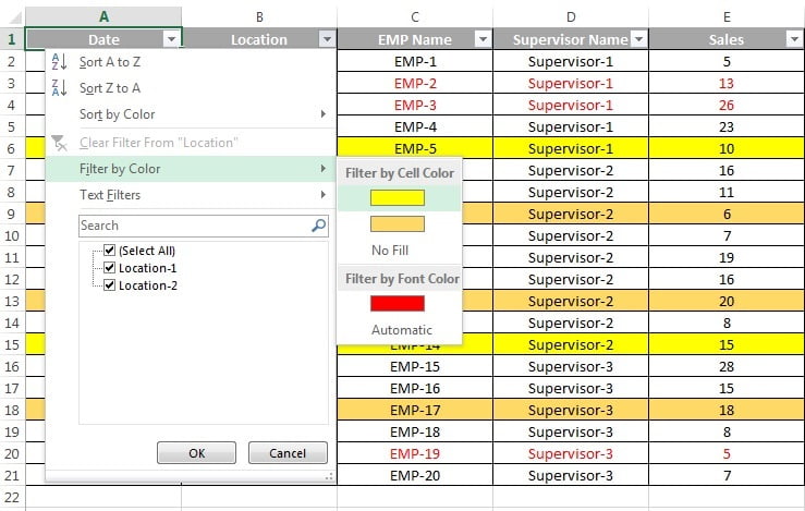
Only the rows with a yellow Date cell remain visible. The row numbers turn blue and the status bar shows how many records were found.

How to filter by font colour
- Clear the previous filter with Data > Sort & Filter > Clear if you want to start fresh.
- Open the drop-down on the Employee column, which contains red text.
- Point to Filter by Color and look under Filter by Font Color.
- Click the red swatch.
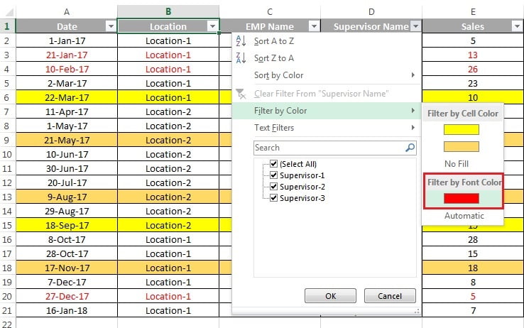
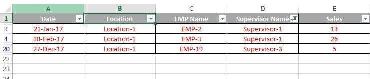
Only rows whose employee name is written in red font are displayed.
Filter by icon and by the selected cell
If a column carries a Conditional Formatting icon set (traffic lights, arrows, flags), the same submenu shows Filter by Cell Icon, listing each icon in the set. Click one to keep only rows with that icon. The quickest route of all is to right-click any coloured cell and choose Filter > Filter by Selected Cell’s Color, Filter by Selected Cell’s Font Color or Filter by Selected Cell’s Icon. This switches AutoFilter on and applies the filter in one step.
Colour filter options compared
| Option | Where | Matches | Works with Conditional Formatting |
|---|---|---|---|
| Filter by Cell Color | Drop-down > Filter by Color | One background fill, or No Fill | Yes |
| Filter by Font Color | Drop-down > Filter by Color | One font colour, or Automatic | Yes |
| Filter by Cell Icon | Drop-down > Filter by Color | One icon from an icon set, or No Cell Icon | Icon sets only |
| Filter by Selected Cell’s Color | Right-click > Filter | The colour of the cell you clicked | Yes |
| Advanced Filter | Data > Advanced | Values only; cannot see colour | No |
Clearing and combining colour filters
To remove the colour filter from one column, open its drop-down and click Clear Filter From “Date”; to remove every filter on the sheet use Data > Clear or press Ctrl+Shift+L twice. Colour filters stack with other filters: filter Date by yellow and then Sales by Number Filters > Greater Than 20 to see highlighted rows with high sales only. Each column allows one colour filter at a time, so “yellow or green” in the same column is not possible; the workaround is in the tips below.
Worked example
A team lead marked the visits that need a follow-up call with a yellow fill in the Date column. Starting from this extract:
| Date | Location | Employee | Sales |
|---|---|---|---|
| 01-Jan (yellow) | Delhi | Ravi | 18 |
| 01-Jan | Mumbai | Neha | 25 |
| 02-Jan (yellow) | Delhi | Amit | 31 |
| 02-Jan (yellow) | Pune | Sara | 12 |
Press Ctrl+Shift+L, open the Date drop-down, point to Filter by Color and click yellow. Three rows remain. Then open the Sales drop-down and choose Number Filters > Greater Than, enter 15 and click OK. Two rows remain: Ravi (18) and Amit (31). A cell holding =SUBTOTAL(103,C2:C5) returns 2, the count of visible rows, and =SUBTOTAL(109,D2:D5) returns 49.
Tips and common mistakes
- One colour per column at a time. To show yellow and green rows together, add a Status column, colour it with Conditional Formatting, and filter that column by its values instead.
- Filter by Color is greyed out when the column contains only one colour or no formatting. Open the drop-down on the column that actually holds the colour.
- Use No Fill to find rows that have not been reviewed yet.
- Totals of filtered rows. Use
=SUBTOTAL(109,E2:E100)or=SUBTOTAL(103,B2:B100)to sum or count only the visible coloured rows. SUM and COUNT include hidden rows. - Shared workbooks. Colours are easy to apply inconsistently across a team; convert them to a Status column with a formula or a macro when the file has several users.
- Theme colours vs standard colours. Two yellows that look alike may be different colours, and each appears as a separate swatch. Pick colours from the same palette row every time.
- Copying the result pastes only visible rows, which is exactly what you want for a follow-up list.
Errors and how to fix them
| Problem | Cause | Fix |
|---|---|---|
| Filter by Color is missing or greyed out | The column has one colour only or none | Use the column that holds the colour; add a second colour or No Fill contrast |
| Two similar swatches appear | Cells were coloured with slightly different shades | Select all marked cells and reapply one fill colour |
| Conditional Formatting colour does not appear | Rule is a colour scale (gradient), which is not filterable | Change to a Highlight Cells rule or icon set, or filter by the underlying value |
| Count is wrong after filtering | COUNT or COUNTA includes hidden rows | Use SUBTOTAL(103, range) or AGGREGATE |
| Rows below a blank row are not filtered | Blank row ends the AutoFilter range | Remove the blank row or select the full range before Ctrl+Shift+L |
Practice exercise
Open the practice file and complete these tasks:
- Colour four Date cells yellow and three Employee names red, then filter each colour in turn.
- Combine the yellow fill filter with a Sales filter of Greater Than 15.
- Right-click a red name and use Filter by Selected Cell’s Font Color.
- Add a Conditional Formatting rule that colours Sales above average green, then filter the Sales column by that green.
- Add
=SUBTOTAL(103,B2:B100)above the table and check it counts only the visible rows.
Key takeaways
- Filter by Color lives in the AutoFilter drop-down and offers cell colour, font colour and cell icon.
- Right-click > Filter by Selected Cell’s Color applies the filter in a single step.
- Only one colour per column can be filtered at once; combine with value filters on other columns for more control.
- Conditional Formatting fills, fonts and icon sets are filterable; colour scales are not.
- Use SUBTOTAL or AGGREGATE to count and total the visible rows.
Related lessons
- Sort and Filter course hub
- Sort by colour
- Text, Number and Date filters
- SUBTOTAL and AGGREGATE with filtered data
- Highlight duplicate or unique values with Conditional Formatting
- Icon sets in Conditional Formatting
- Microsoft Support: Filter data in a range or table
Frequently asked questions
Can I filter by two colours at the same time?
Not in one column. Filter by one colour, or apply the colours through Conditional Formatting driven by a status column and filter that column by its values instead. You can, however, filter one column by colour and a different column by another colour at the same time.
Does filter by colour work with conditional formatting?
Yes. Fills, font colours and icon sets produced by Conditional Formatting appear in the Filter by Color submenu exactly like manual formatting. The exception is colour scales, whose gradient colours are not listed, so filter by the value that drives the scale instead.
How do I count the coloured rows after filtering?
Use =SUBTOTAL(103,A2:A100) for a count or =SUBTOTAL(109,E2:E100) for a sum. SUBTOTAL with function numbers 101 to 111 ignores rows hidden by a filter, so the result reflects only the visible colour. AGGREGATE with option 5 does the same job.
Why is Filter by Color greyed out?
Excel enables the command only when the column contains at least two different formats, for example yellow and No Fill. If every cell has the same colour, or the colour sits in a different column, the option is disabled. Open the drop-down of the column that actually holds the colour.
Can I filter by colour with a formula instead?
Excel has no built-in worksheet function that reads a cell’s colour. The reliable alternatives are a Status column that drives the colour through Conditional Formatting, the legacy GET.CELL macro function in a defined name, or a short VBA user-defined function that returns Interior.ColorIndex.
Want the finished version? Ready-made Excel dashboards, trackers and VBA systems are available at NextGenTemplates.com.