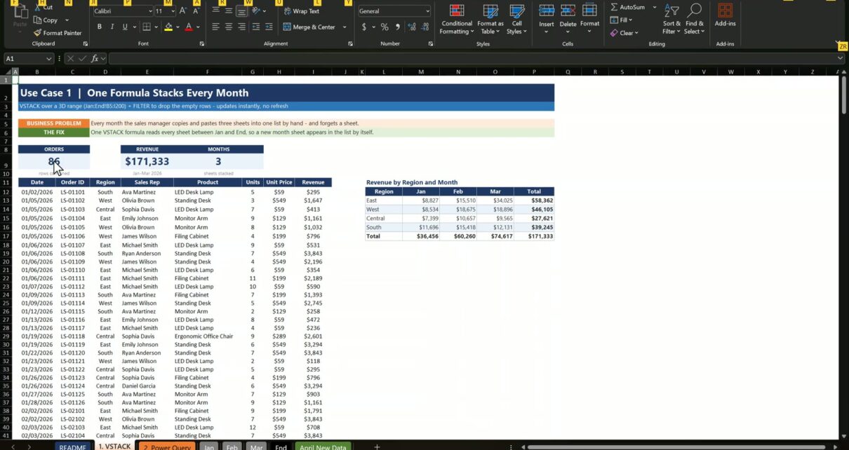
Every month the sales manager copies the month tabs into one list by hand, and one day a tab gets missed and the report is wrong. In this tutorial you combine monthly sales reports in Excel with two methods, a single VSTACK formula and Power Query, so the combined list builds itself. The example is Lone Star Office Supply in Dallas, Texas: three months of orders become one list of 86 orders and $171,333 in revenue, and when April arrives it becomes 116 orders and $238,455 without copying one row.
⬇️ Download the Free Practice Files
Watch the Video Tutorial
Video Overview
The fifteen-minute video opens with the finished file: drag the April tab in front of the End tab and the formula list jumps from 86 to 116 orders, while the Power Query list waits for Refresh All and then shows the same numbers. Then you build both methods from the practice file in three use cases. Use case one is the VSTACK formula with an End bookend tab, LET and FILTER to remove empty rows, three cards and a Region by Month grid. Use case two is Power Query: month tables, a short M query, a table loaded to the sheet and a SUMIFS grid. Use case three adds April and compares the two methods.
What You Will Build
- One VSTACK formula that stacks every month tab between Jan and End.
- A clean list with LET, FILTER and CHOOSECOLS that drops the empty rows.
- Live cards for orders, revenue and number of months, plus a Region by Month grid.
- A Power Query that appends every month table and loads it as PQ_AllSales.
- A test with April: 30 new orders added without copying anything.
The Practice Files and the Data
Each month tab has the same columns in B to I: Date, Order ID, Region, Sales Rep, Product, Units, Unit Price and Revenue, with the header in row 4. January has 26 orders, February 28 and March 32. The Practice file has the layout, the three month tabs and an April New Data tab. The End tab, the formulas, the query and the tables are empty, so you build them on camera. The Solution file has everything working. All names and numbers are fictional example data.
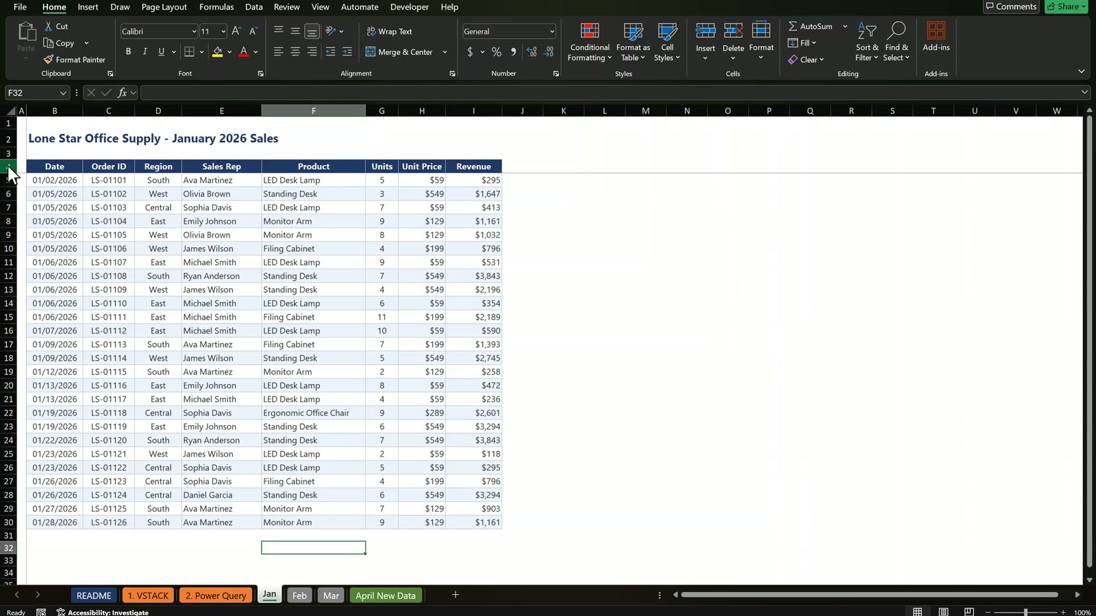
Use Case 1: One VSTACK Formula
The End tab bookend
Click the March tab, add a new blank tab after it and name it End. Keep it empty. Excel can read the same range on every tab from Jan to End in one go, so any month tab between those two is included.
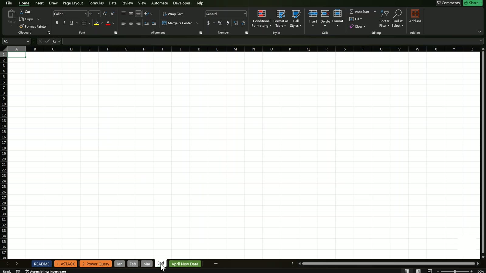
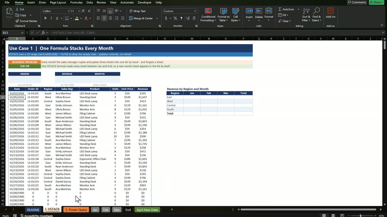
The formula and the zero rows
On the VSTACK tab select B12 and type the formula below. Click Jan, hold Shift and click End to group the tabs, then type the range B5:I200 so every month has room to grow.
=VSTACK(Jan:End!B5:I200)
The result has rows of zeros after the last order of every month, because VSTACK reads all 200 rows and empty cells come back as 0, not blank.
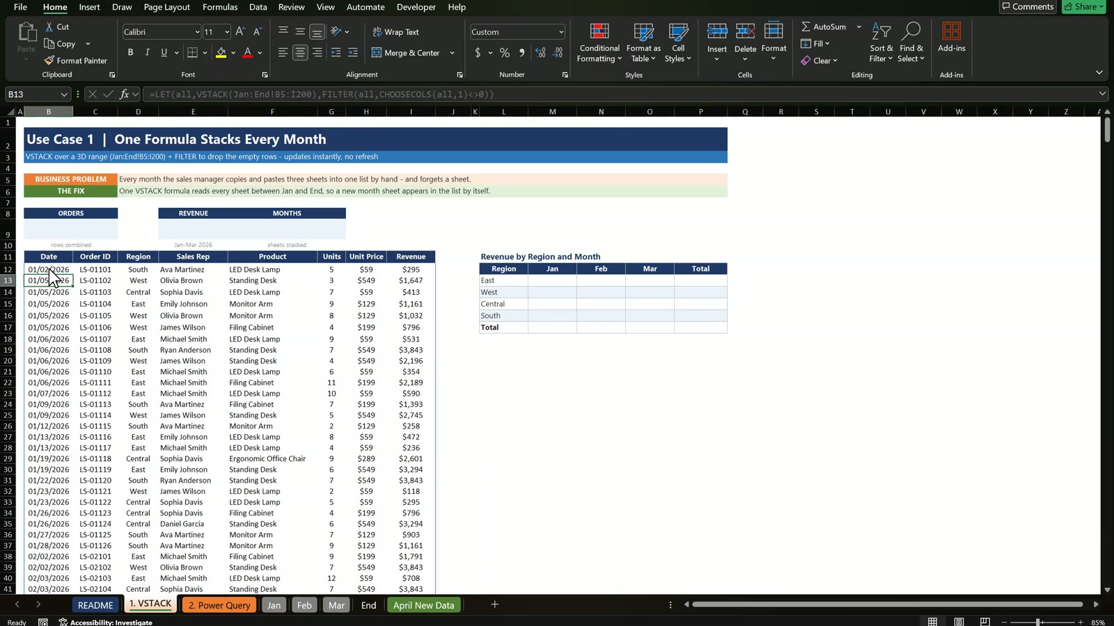
LET and FILTER
Give the whole list a short name with LET and keep only the rows where the date is not zero:
=LET(all,VSTACK(Jan:End!B5:I200),FILTER(all,CHOOSECOLS(all,1)<>0))
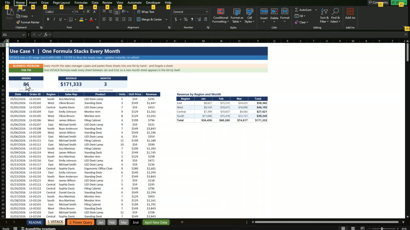
You get 86 clean rows from 01/02/2026 to the end of March in one cell, so nobody can delete a row in the middle by mistake.
Cards and the Region by Month grid
The hash sign refers to the whole spill range, however long it gets. The three cards are:
- Orders:
=ROWS(B12#)returns 86. - Revenue:
=SUM(CHOOSECOLS(B12#,8))returns $171,333. - Months:
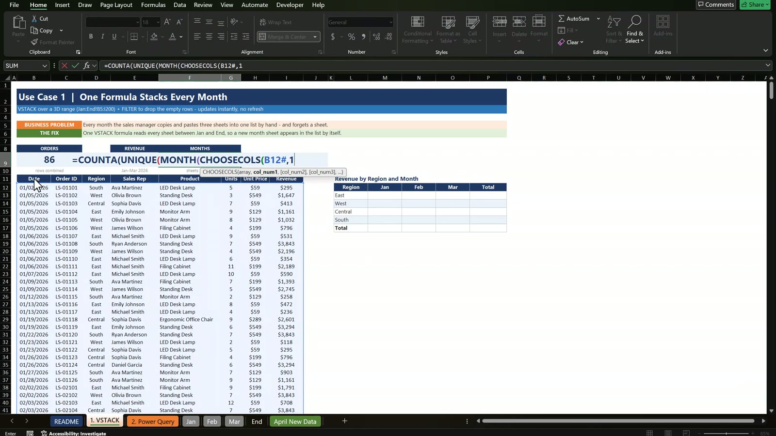
=COUNTA(UNIQUE(MONTH(CHOOSECOLS(B12#,1))))returns 3.
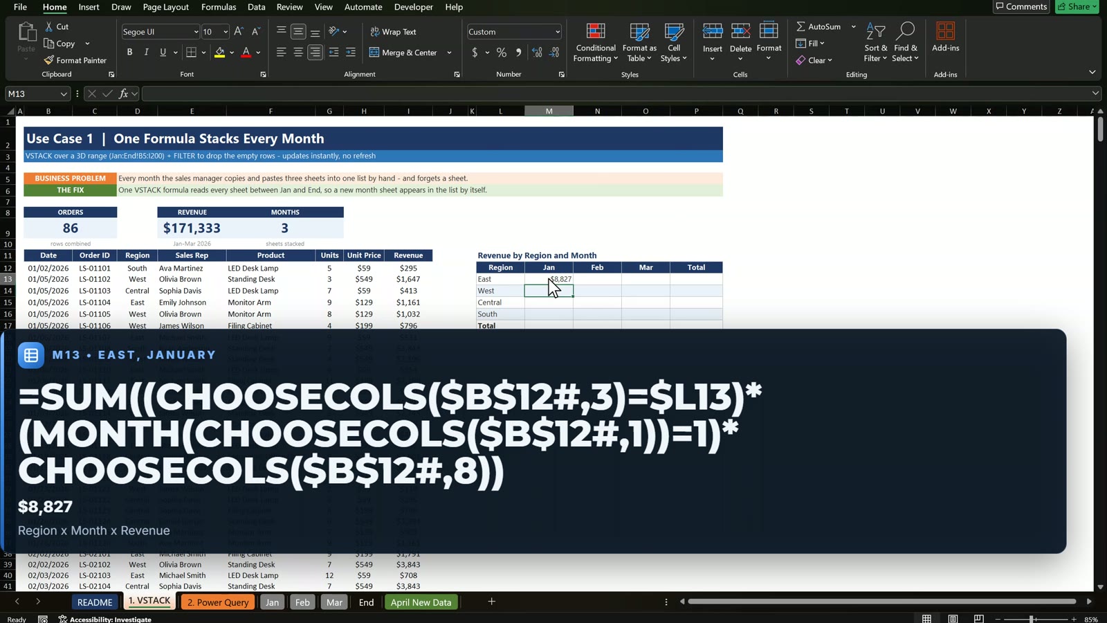
Gotcha: SUMIFS only accepts real cell ranges, so it gives an error on a list made by a formula. Multiply the conditions inside SUM instead. In M13 (East, January):
=SUM((CHOOSECOLS($B$12#,3)=$L13)*(MONTH(CHOOSECOLS($B$12#,1))=1)*CHOOSECOLS($B$12#,8))
East sold $8,827 in January. Change the 1 to 2 and 3 for February and March, fill down with Ctrl+D and use Alt+= for the totals. The grand total matches the card at $171,333.
Use Case 2: Power Query
Power Query does the same job, also works in older Excel versions, sets the data types and handles 100,000 rows or more. It works best with tables, so on each month tab click inside the data, press Ctrl+T and name the tables tblJan, tblFeb and tblMar. The tbl prefix matters because the query keeps every table whose name starts with it.
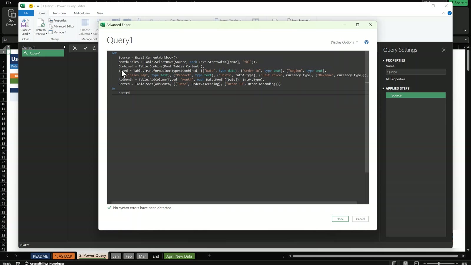
On the Power Query tab choose Data, Get Data, From Other Sources, Blank Query, then open the Advanced Editor and paste this query:
let
    Source = Excel.CurrentWorkbook(),
    MonthTables = Table.SelectRows(Source, each Text.StartsWith([Name], "tbl")),
    Combined = Table.Combine(MonthTables[Content]),
    Typed = Table.TransformColumnTypes(Combined, {{"Date", type date}, {"Order ID", type text}, {"Region", type text}, {"Sales Rep", type text}, {"Product", type text}, {"Units", Int64.Type}, {"Unit Price", Currency.Type}, {"Revenue", Currency.Type}}),
    AddMonth = Table.AddColumn(Typed, "Month", each Date.Month([Date]), Int64.Type),
    Sorted = Table.Sort(AddMonth, {{"Date", Order.Ascending}, {"Order ID", Order.Ascending}})
in
    Sorted
Excel.CurrentWorkbook lists every table in the file, Table.SelectRows keeps the ones starting with tbl, Table.Combine stacks them, the types are set, a Month column is added and the list is sorted by date and order ID. Name the query AllSales and you see 9 columns and 86 rows.
Close and Load, and the table name gotcha
Choose Close and Load To, keep Table, pick Existing worksheet and click B11 on the Power Query tab. Then rename the output table in Table Design to PQ_AllSales. Never start the output name with tbl: the query would read its own output on the next refresh and every row would appear twice. Format Unit Price and Revenue with $#,##0 (Ctrl+1, Custom).
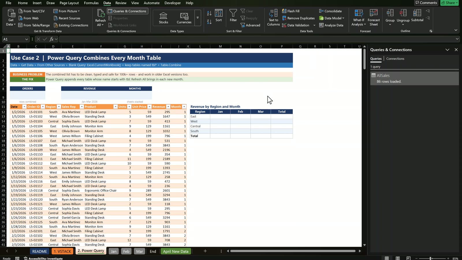
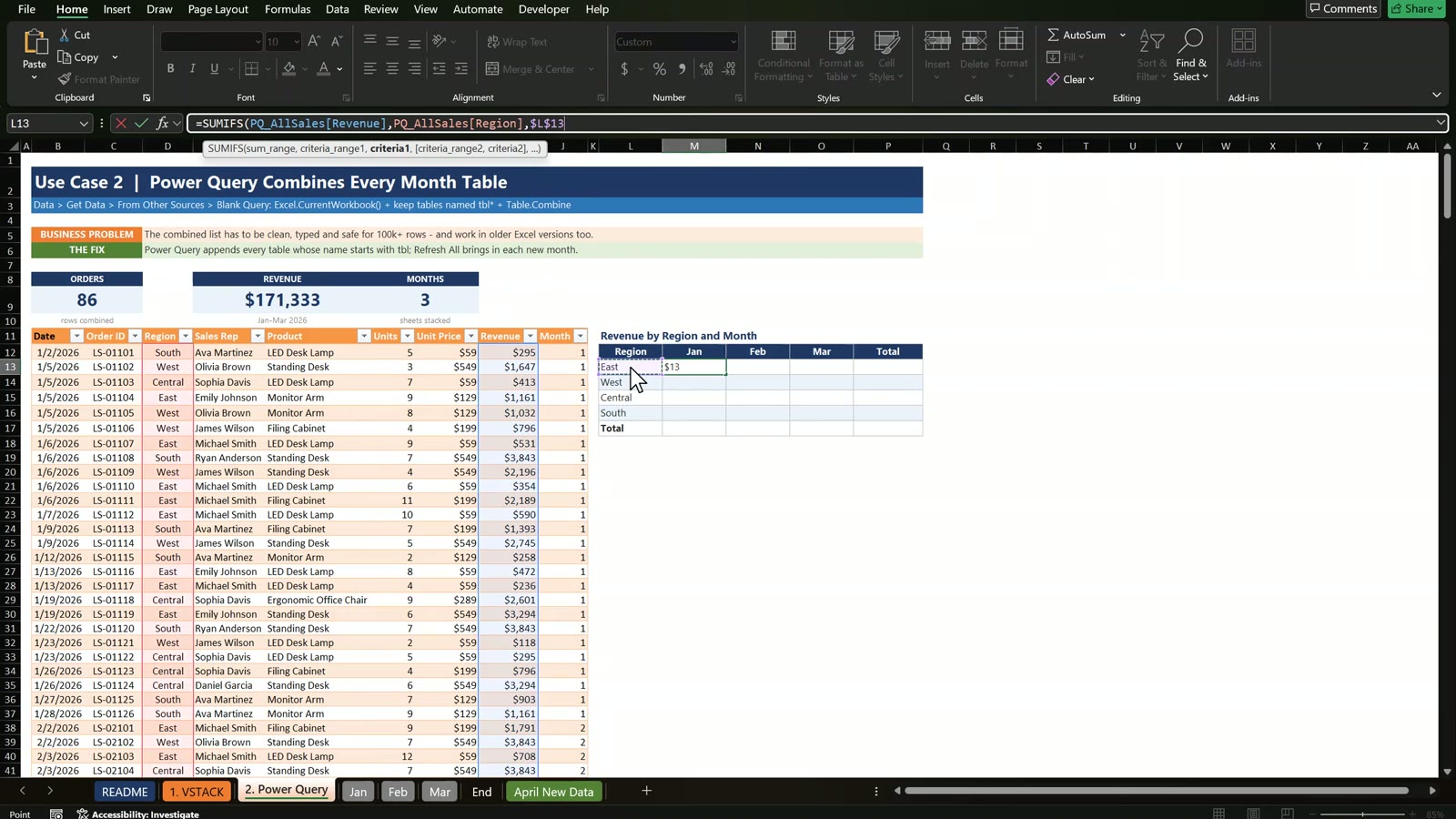
The cards use the table: =ROWS(PQ_AllSales), =SUM(PQ_AllSales[Revenue]) and =COUNTA(UNIQUE(PQ_AllSales[Month])). Here SUMIFS works because a table column is a real range:
=SUMIFS(PQ_AllSales[Revenue],PQ_AllSales[Region],$L13,PQ_AllSales[Month],1)
Use Case 3: The Real Test, Add April
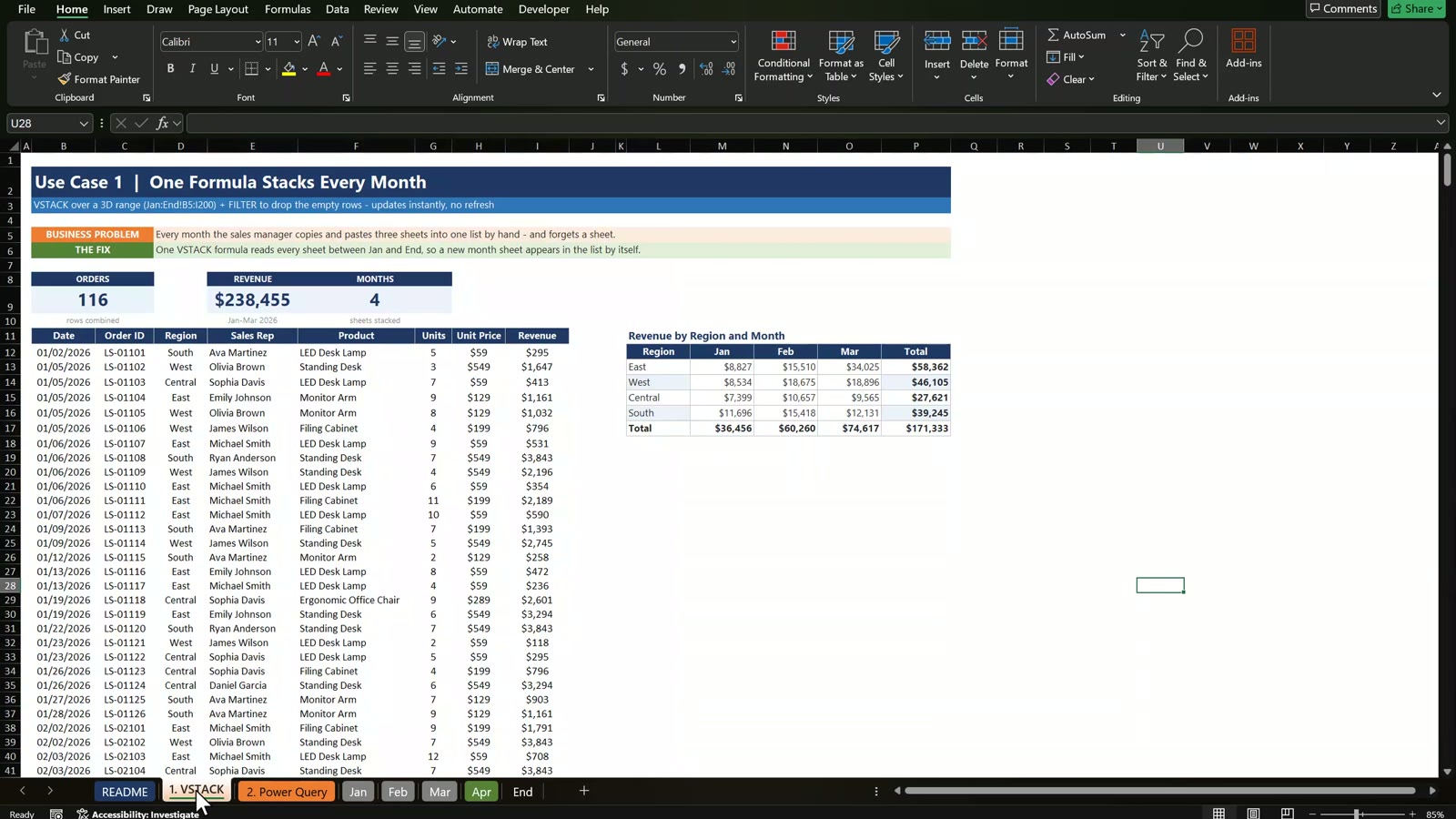
The April New Data tab has 30 new orders with the same columns. Press Ctrl+T, name the table tblApr and rename the tab to Apr. The formula tab still shows 86 orders because Apr sits after End, outside the range. This is the third gotcha: every month must sit between Jan and End. Drag the Apr tab in front of End and the formula list instantly shows 116 orders, $238,455 and four months.
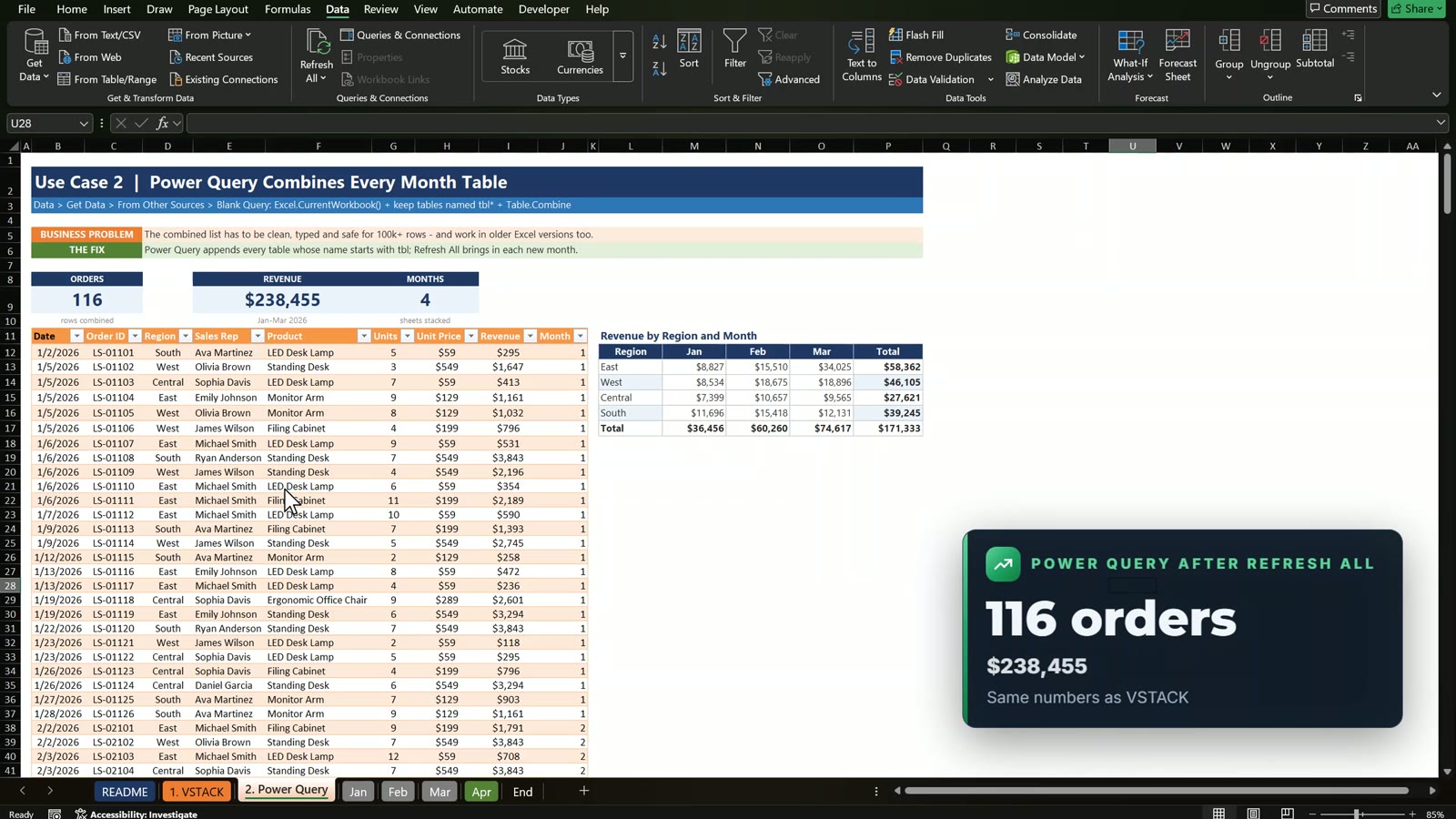
The Power Query tab still shows 86 until you click Data, Refresh All. Then it also shows 116 orders and $238,455. To skip the click, open the query properties and tick Refresh data when opening the file.
VSTACK or Power Query: Which Should You Use?
| Method | Strength | Limit | Use it for |
|---|---|---|---|
| Formula | One cell, no refresh, updates instantly | Excel 365 / 2024 only, same layout on every tab | A small monthly report |
| Power Query | Excel 2016+, sets data types, cleans messy data, 100,000+ rows | Needs Refresh All (or refresh on open) | Big or messy data |
For a small monthly report I use the formula. For big or messy data I use Power Query. If you want the numbers in a finished dashboard layout, see the Channel Sales Dashboard in Excel on Next Gen Templates, and to learn formulas like these in depth join the Excel + AI Mastery: 100 Essential Formulas course.
Related Tutorials
- Billing System in Excel: Build an Invoice System Step by Step
- How to Make a Production Tracker in Excel
- Gantt Chart in Excel 2026 Step by Step
Frequently Asked Questions
How do I combine monthly sales reports in Excel into one list?
Use one VSTACK formula over a 3D range, for example =LET(all,VSTACK(Jan:End!B5:I200),FILTER(all,CHOOSECOLS(all,1)<>0)), or load every month table with Power Query. Both stack the sheets one under the other and update when you add a month.
What does the End sheet do in the VSTACK formula?
It is an empty bookend. A 3D reference reads every sheet between Jan and End, so any new month tab placed in front of End is included automatically. A sheet placed after End is ignored.
Why does VSTACK return rows of zeros?
The range B5:I200 is read on every sheet, and empty cells come back as 0, not blank. Wrap the result in FILTER and keep only the rows where the date column is not 0.
Why does SUMIFS give an error on the VSTACK result?
SUMIFS needs real cell ranges and does not accept an array made by CHOOSECOLS. Use SUM with the conditions multiplied inside it, or point SUMIFS at a Power Query table column.
Does Power Query refresh automatically?
Not by default. Click Data, Refresh All after adding a month, or open Query Properties and tick Refresh data when opening the file.
Why must the Power Query output table not start with tbl?
The query keeps every table whose name starts with tbl. If the output table also starts with tbl, the query reads its own result on the next refresh and every row appears twice. Name it PQ_AllSales.
Which is better, VSTACK or Power Query?
VSTACK is one formula and updates instantly, but needs Excel 365 or Excel 2024 and the same layout on every sheet. Power Query works in Excel 2016 and later, sets data types, cleans messy data and handles 100,000 rows or more, but needs a refresh.
Is the practice file free?
Yes. The zip has the Practice and Solution workbooks for a fictional office furniture business in Dallas, Texas. All names and numbers are example data.
Download the Free Practice Files
⬇️ Download the Free Practice Files
By PK, An Excel Expert. Lone Star Office Supply and all names and numbers are fictional example data for learning.
Conclusion
One VSTACK formula or one Power Query turns a pile of monthly tabs into a single list that updates when you add a month. Download the free files, build both methods along with the video and compare with the Solution file if you get stuck.