Filter Data in Excel: Apply, Search and Clear Filters

Part of the free Module 4: Sort and Filter · Lesson 3 of 11 · Full Excel course

Updated on 5 September 2026 · Works in Excel 365, 2021, 2019 and 2016 unless noted.

To filter data in Excel, click one cell in your table and press Ctrl+Shift+L (or choose Data > Sort & Filter > Filter). Drop-down arrows appear on every header; open one, untick (Select All), tick the values you want and click OK. Excel hides every non-matching row without deleting anything, and you can clear the filter at any time.

Table of Contents

What a filter does and when to use it

Filtering is temporary and non-destructive. Each drop-down lists the unique values in its column with a check box, so you can show one supervisor, two locations, or every employee except one. Hidden rows keep their row numbers, which turn blue, and reappear the moment the filter is cleared. Filters on different columns combine with AND logic: Supervisor-1 and Location Delhi.

Use a filter to review a subset of records, to copy only the visible rows to another sheet, to delete matching rows safely, or to feed a SUBTOTAL formula that totals only what is visible. When the same subset is needed every day, the FILTER function or an Excel Table with slicers is a better long-term tool.

The sample data

The lesson uses the daily sales list from the course practice file: Date, Location, Supervisor, Employee and Sales, with one header row and no blank rows.

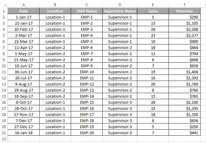
Sales data set with Date, Location, Supervisor, Employee and Sales columns before you filter data in Excel — Data set before applying the filter

How to apply a filter in Excel

Click any single cell inside the data range. Excel detects the surrounding block automatically as long as there are no blank rows or columns.
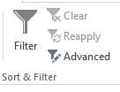
Go to Data > Sort & Filter > Filter, or press Ctrl+Shift+L. Drop-down arrows appear on every header cell.

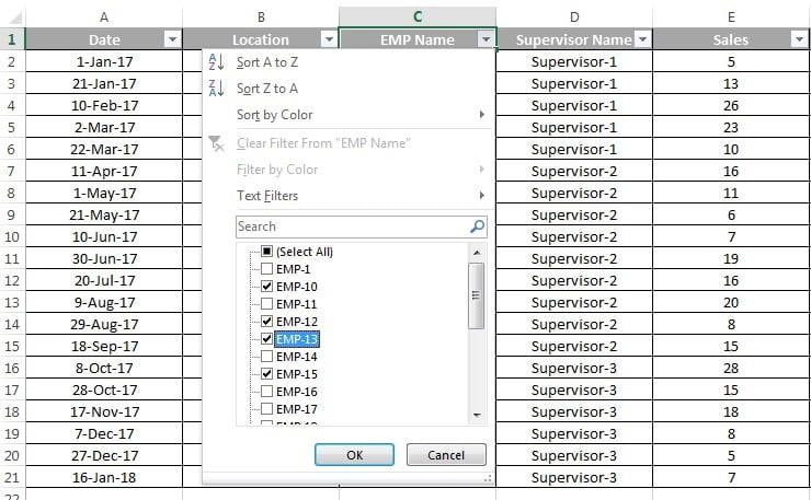
Filter button in the Sort and Filter group of the Excel Data tab — Filter button on the Data tab

Open the drop-down on the column you want to filter, for example Supervisor. The keyboard route is to select the header cell and press Alt+Down Arrow.
Untick (Select All) to clear every check box, then tick only the items you want to see.
Click OK. Only matching rows remain visible, the arrow changes to a funnel icon and the status bar reports “x of y records found”.

Excel filter drop-down with Select All unticked and one supervisor ticked to filter the data — Ticking items in the filter drop-down

Repeat on a second column to narrow the result further. Every column that has an active filter shows the funnel icon, so you can see at a glance which conditions are in force.

How to clear a filter

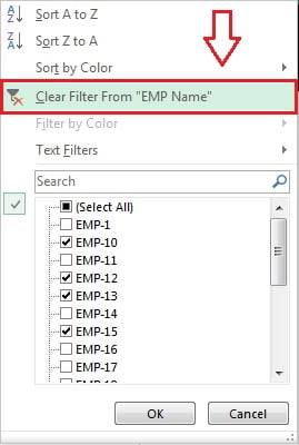
One column: open its drop-down and click Clear Filter From “Supervisor”.
All columns, keep the arrows: choose Data > Sort & Filter > Clear (Alt, A, C).
Remove the filter completely: press Ctrl+Shift+L again or click Data > Filter to toggle the arrows off. All rows reappear.
Reapply (Data > Sort & Filter > Reapply, or Ctrl+Alt+L) re-runs the current filter after you edit values, because AutoFilter does not refresh itself.

Clear Filter From command in the Excel column drop-down used to remove a filter from one field — Clear Filter From a single column

Filter by search

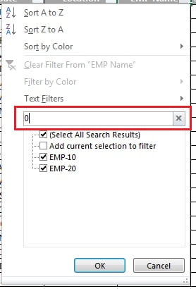
When a column has hundreds of unique values, ticking boxes is slow. Type part of a value in the Search box at the top of the drop-down and the list shrinks to matching items only; press Enter or click OK to apply. The search is not case sensitive and matches anywhere in the text, so del finds Delhi and Model. To add a second search to an existing filter, run the new search and tick Add current selection to filter before clicking OK.

Search box inside the Excel filter drop-down narrowing the list of items to filter by — Filter by typing in the Search box

Filter shortcuts and wildcards

Action	Shortcut or symbol	Notes
Turn filter arrows on or off	Ctrl+Shift+L	Works from any cell in the range
Open the drop-down of the selected header	Alt+Down Arrow	Then type to jump to the search box
Clear all filters, keep arrows	Alt, A, C	Same as Data > Clear
Reapply the current filter	Ctrl+Alt+L	Refreshes after edits
Any number of characters	*	`Sup*` finds Supervisor-1, Supervisor-2
Exactly one character	?	`?-1` matches A-1, B-1
A literal * or ?	~* or ~?	Tilde escapes the wildcard

Worked example

A regional manager needs the Delhi sales handled by Supervisor-1 so she can check them before month end. With this extract:

Date	Location	Supervisor	Sales
01-Jan	Delhi	Supervisor-1	4,200
01-Jan	Mumbai	Supervisor-1	5,100
02-Jan	Delhi	Supervisor-2	6,300
02-Jan	Delhi	Supervisor-1	2,900

Press Ctrl+Shift+L, open the Location drop-down, untick (Select All), tick Delhi and click OK. Three rows remain. Open the Supervisor drop-down, tick only Supervisor-1 and click OK. Two rows remain (4,200 and 2,900), and the status bar reads “2 of 4 records found”. A cell containing =SUBTOTAL(109,D2:D5) shows 7,100, the total of the visible rows only.

Tips and common mistakes

A blank row breaks the filter. Rows below an empty row are ignored. Select the entire range before pressing Ctrl+Shift+L, or remove the blank row.
Totals include hidden rows. SUM adds everything; use =SUBTOTAL(109,E2:E100) or AGGREGATE to total only visible cells (see the SUBTOTAL and AGGREGATE lesson).
Copy visible rows only. Copying a filtered range pastes only the visible rows, but pasting into a filtered range fills hidden rows too. Filter, then paste into a clean sheet.
Convert to a Table (Ctrl+T) to get permanent filter arrows, banded rows and ranges that grow with the data.
One AutoFilter per sheet. A worksheet can hold only one AutoFilter range unless the data is in Tables.
Filters do not refresh themselves. After editing values, press Ctrl+Alt+L to reapply.
Check the drop-down for “(Blanks)”. Unticking it is the quickest way to hide empty rows.

Errors and how to fix them

Problem	Cause	Fix
Filter arrows appear on the wrong row	Active cell was outside the data, or the header row is not the first row of the block	Click a cell inside the data or select the range including the header first
Some rows are missing from the drop-down list	Blank row splits the range, or the list has more than 10,000 unique items	Delete blank rows; use the Search box for long lists
Filter button is greyed out	Sheet is protected, workbook is shared, or several sheets are grouped	Unprotect the sheet or ungroup the sheets
Numbers and text mixed in the list	Some numbers are stored as text	Convert with Text to Columns, then reapply
Filter shows old results after edits	AutoFilter does not recalculate	Press Ctrl+Alt+L or Data > Reapply

Practice exercise

Open the practice file and complete these tasks:

Switch the filter on with Ctrl+Shift+L and show only Supervisor-1.
Add a second filter on Location and confirm that both conditions apply at once.
Use the Search box to find every employee whose name contains “an”, then add a second search with Add current selection to filter.
Enter =SUBTOTAL(109,E2:E100) above the Sales column and watch it change as you filter.
Clear the Location filter only, then clear all filters with Alt, A, C.

Key takeaways

Ctrl+Shift+L turns AutoFilter on and off; the arrows sit on the header row of the block that contains the active cell.
Filters hide rows, never delete them, and filters on several columns combine with AND.
The Search box with * and ? wildcards is faster than ticking boxes in long lists.
Clear one column from its drop-down, clear all with Data > Clear, and reapply with Ctrl+Alt+L after edits.
Use SUBTOTAL, not SUM, to total filtered data.

Related lessons

Frequently asked questions

What is the shortcut for filter in Excel?

Ctrl+Shift+L toggles the AutoFilter arrows on and off. Alt+Down Arrow opens the drop-down of the selected header cell, Alt, A, C clears all filters while keeping the arrows, and Ctrl+Alt+L reapplies the current filter after you change values.

Why does my filter not include all rows?

There is usually a blank row or a merged cell inside the data, so Excel stopped the range early. Select the whole range manually before applying the filter, or delete the blank row. If rows were added after filtering, press Ctrl+Alt+L to reapply.

How do I filter for multiple values in one column?

Open the drop-down, untick (Select All) and tick each value you need, then click OK. For long lists, type each search term in turn in the Search box and tick Add current selection to filter before clicking OK so the earlier choices are kept.

How do I copy only the filtered rows?

Select the filtered range, press Ctrl+C and paste on a new sheet. Excel copies visible rows only. If hidden rows come across, select the range, press Alt+; (Select Visible Cells) before copying. Never paste into a filtered range, because hidden rows receive data too.

Does a filter change the data or formulas?

No. Filtering only hides rows. Formulas keep calculating on all rows, which is why SUM still includes hidden values and SUBTOTAL or AGGREGATE are the functions to use for visible-only totals.

Want the finished version? Ready-made Excel dashboards, trackers and VBA systems are available at NextGenTemplates.com.