Text, Number and Date Filters in Excel: AutoFilter Options Guide

Part of the free Module 4: Sort and Filter · Lesson 4 of 11 · Full Excel course

Updated on 5 September 2026 · Works in Excel 365, 2021, 2019 and 2016 unless noted.

Text, number and date filters in Excel are the condition-based options inside the AutoFilter drop-down. Instead of ticking individual items, you describe what you want: names that begin with “S”, sales greater than 20, or dates in the last month. Excel shows Text Filters, Number Filters or Date Filters depending on the data type of the column, and every option opens the Custom AutoFilter dialog where you can combine two conditions with And or Or.

How Excel decides between Text, Number and Date Filters

When you open a filter arrow, Excel looks at the values in that column. If most cells hold text, the submenu is Text Filters. If most cells hold numbers, it becomes Number Filters. If most cells hold true dates (serial numbers formatted as dates), it becomes Date Filters and the checklist is grouped into a year, month and day tree.

This is why Greater Than sometimes appears to be missing. Numbers imported as text, or dates typed into text-formatted cells, are treated as text, so only Text Filters are offered. Convert the values and the menu changes; the errors table below gives the fixes.

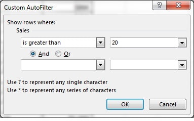
Whatever the type, choosing a condition opens the Custom AutoFilter dialog. It has two rows of criteria joined by And or Or, and text criteria accept the wildcards * (any number of characters) and ? (exactly one character).

Filter types compared

Filter type	Options in the submenu	Example
Text Filters	Equals, Does Not Equal, Begins With, Ends With, Contains, Does Not Contain, Custom Filter	Employee begins with “S” and does not contain “3”
Number Filters	Equals, Does Not Equal, Greater Than, Greater Than Or Equal To, Less Than, Less Than Or Equal To, Between, Top 10, Above Average, Below Average, Custom Filter	Sales between 10 and 25; top 5 percent of Sales
Date Filters	Equals, Before, After, Between, Tomorrow, Today, Yesterday, Next/This/Last Week, Next/This/Last Month, Next/This/Last Quarter, Next/This/Last Year, Year to Date, All Dates in the Period, Custom Filter	Date is in Last Month; all dates in Quarter 1 of any year

Text Filters: Equals, Begins With, Contains and more

Open the drop-down on a text column such as Employee and point to Text Filters.

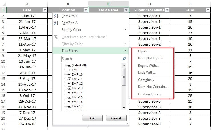
• Equals and Does Not Equal: exact match of the whole cell. Not case-sensitive, so “smith” matches “Smith”.
• Begins With and Ends With: match the first or last characters. Useful for codes such as “INV-” or file extensions.
• Contains and Does Not Contain: match anywhere in the cell.
• Custom Filter: opens the dialog with both rows blank.

1. Select any cell in the data and press Ctrl+Shift+L if the filter arrows are not yet showing.
2. Open the drop-down on Employee and click Text Filters > Equals.
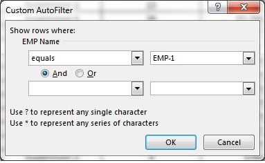
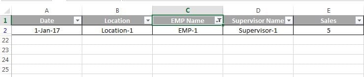
3. In the Custom AutoFilter dialog type the name, or pick it from the value list on the right, and click OK.

Number Filters: Greater Than, Between, Top 10 and Above Average

On a numeric column such as Sales the submenu becomes Number Filters.

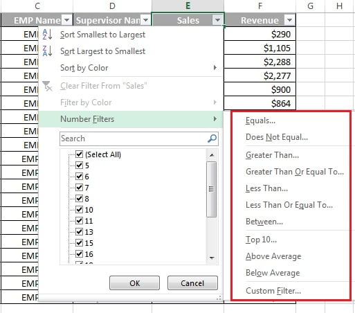
• Equals, Does Not Equal, Greater Than, Greater Than Or Equal To, Less Than and Less Than Or Equal To: single comparisons against one value.
• Between: two boundaries, and both are inclusive. Between 10 and 25 keeps 10 and 25.
• Top 10: opens its own dialog. Choose Top or Bottom, any number from 1 to 500, and Items or Percent. Top 5 Percent keeps the highest 5 percent of the rows by value.
• Above Average and Below Average: compare each value with the mean of the whole column, ignoring filters on other columns.

1. Open the drop-down on Sales and click Number Filters > Greater Than.
2. Type 20 in the box and click OK. Only rows with Sales above 20 remain.
3. To keep a range instead, reopen the dialog, set the second row to is less than or equal to 50 and leave And selected.

Date Filters and the year, month and day tree

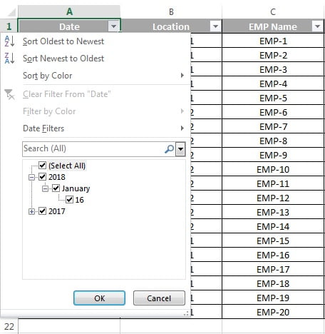
A true date column is grouped automatically in the checklist. Each year has a plus sign; expand it to see months, and expand a month to see days. Tick a month to include every day in it with one click, or untick a year to remove it entirely. This grouping only appears when the cells hold real dates.

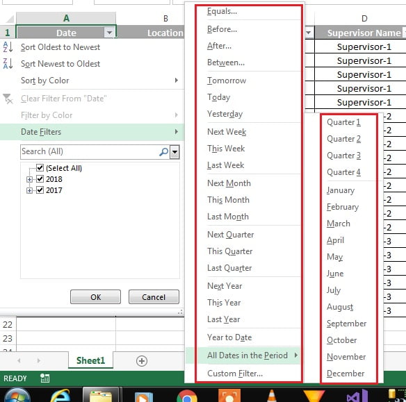
The Date Filters submenu adds two kinds of condition. Equals, Before, After and Between take fixed dates that you type or pick from the calendar button. The dynamic options, Tomorrow, Today, Yesterday, Next/This/Last Week, Month, Quarter and Year, plus Year to Date, are evaluated against your computer’s date each time the filter is applied or reapplied. A “This Month” filter saved in a report therefore stays current when you reopen the file next month and press Ctrl+Alt+L.

All Dates in the Period is different again: it picks a quarter or a month from every year in the column. Choosing Quarter 1 keeps January to March of 2024, 2025 and 2026 together, which is ideal for year-on-year comparisons.

Custom AutoFilter: And, Or and wildcards

Every condition leads to the same dialog, so it pays to know it well. The first row holds the operator and value you chose from the menu. The second row is optional. And keeps rows that meet both conditions; Or keeps rows that meet either. In text criteria, * stands for any run of characters and ? for one character, so Emp?? matches Emp01 but not Emp001, and *-1 matches any value ending in “-1”. To search for a literal asterisk or question mark, type a tilde first: ~*.

The dialog allows only two conditions per column; a third needs a helper column or the Advanced Filter. Conditions on different columns are always combined with And.

Worked example

Use this small sales list, which matches the layout of the course practice file.

Employee	Sales	Date
Emp-1	18	03 Jul 2026
Emp-2	32	15 Jul 2026
Emp-3	27	02 Aug 2026
Emp-4	9	19 Aug 2026
Emp-5	41	28 Aug 2026
Emp-6	22	04 Sep 2026

Goal: list the employees who sold more than 20 in August 2026, with today’s date being 5 September 2026.

1. Click any cell in the list and press Ctrl+Shift+L.
2. Open the Sales drop-down, choose Number Filters > Greater Than, type 20 and click OK. Emp-1 and Emp-4 disappear.
3. Open the Date drop-down and choose Date Filters > Last Month. Because today is in September, Excel keeps August only.

Result: two rows remain, Emp-3 (27) and Emp-5 (41), and the status bar reads “2 of 6 records found”. Switch the date filter to Year to Date and Emp-2 and Emp-6 return.

Tips and common mistakes

• Check the submenu name first. If a number column shows Text Filters, the values are text. Fix the data rather than fighting the filter.
• Between is inclusive. Between 10 and 25 keeps rows equal to 10 and 25. Use Greater Than and Less Than if you need exclusive limits.
• Top 10 works on values, not rows. Ties are all kept, so “Top 3 Items” can return four rows if two values are equal.
• Above Average ignores other filters. The average is always calculated on the full column. For an average of visible rows, use SUBTOTAL in a helper column and filter on that.
• Dynamic date filters follow the system clock. “Last Quarter” uses calendar quarters, not your financial year.
• Reapply after editing data. Filters do not refresh on their own. Press Ctrl+Alt+L or click Data > Reapply.

Errors and how to fix them

Symptom	Cause	Fix
Date Filters missing; dates listed flat with no year tree	Dates are stored as text, often after a CSV import	Select the column, click Data > Text to Columns, choose Date in step 3 and click Finish
Number Filters missing on a numeric column	Numbers stored as text (green triangle in the corner)	Type 1 in a spare cell, copy it, select the column and use Paste Special > Multiply, or use Text to Columns
Date tree missing although dates are real	Grouping switched off in options	File > Options > Advanced, tick Group dates in the AutoFilter menu
Contains “S*” returns nothing	The asterisk is being read as a wildcard	Type S~* to match a literal asterisk
Filter returns no rows although matches exist	Leading or trailing spaces in the data, or a filter left on another column	Clean with Find and Replace or TRIM, and click Data > Clear to remove all filters

Practice exercise

Download the practice workbook Sort-and-Filter.xlsx and try these tasks on the Employee, Sales and Date columns.

1. Filter Employee to names that begin with “E” and do not contain “3” using one Custom AutoFilter dialog.
2. Show only Sales between 10 and 25, then switch to Top 10 with 5 Percent and note how many rows remain.
3. Filter Date to Last Month, then to All Dates in the Period > Quarter 3, and compare the two results.
4. Combine all three: Employee begins with “E”, Sales above average, Date year to date.
5. Convert the Date column to text with Text to Columns, reopen the filter and confirm that Date Filters has disappeared. Convert it back.

Key takeaways

• The AutoFilter submenu shows Text, Number or Date Filters based on the data type of the column, so the menu itself tells you whether your data is stored correctly.
• Every condition opens the Custom AutoFilter dialog, which accepts two criteria joined by And or Or, plus the wildcards * and ?.
• Number filters include Between (inclusive), Top 10 by items or percent, and Above or Below Average.
• Dynamic date filters such as Today, Last Month and Year to Date follow the system date, so reports stay current when reapplied.
• All Dates in the Period compares the same month or quarter across every year.
• Filters on different columns always combine with And.

Related lessons

• Sort and Filter course hub
• Data Filter in Excel: apply, clear and search AutoFilter
• Filter by Colour in Excel
• Advanced Filter in Excel: criteria range and unique records
• SORT, SORTBY, FILTER and UNIQUE functions
• FILTER function for formula-based filtering, and COUNTIF for counting with wildcards
• Microsoft Support: Filter data in a range or table

Frequently asked questions

Why do I see Text Filters instead of Number Filters in Excel?

The column contains numbers stored as text, which often happens after an import or a copy from a web page. Select the column, use Data > Text to Columns > Finish, or copy a cell containing 1 and use Paste Special > Multiply. Reopen the drop-down and it will now show Number Filters.

Why are Date Filters missing from the filter menu?

Excel only offers Date Filters and the year-month tree when the cells hold real dates. Dates typed into text-formatted cells, or imported as text, are treated as words. Convert them with Text to Columns, choosing Date in the last step, or use the DATEVALUE function in a helper column and paste the values back.

How do I filter dates by month in Excel?

Open the date column drop-down and tick the month under its year in the grouped checklist. To keep the same month from every year, choose Date Filters > All Dates in the Period and pick the month. For a rolling report choose This Month or Last Month, which update against the system date.

Can I use wildcards in an Excel text filter?

Yes. In the Custom AutoFilter dialog, * stands for any number of characters and ? for exactly one, so S*-1 matches S-1 and Sales-1, and Emp?? matches five-character codes only. To match a literal asterisk or question mark, put a tilde in front of it, for example ~?.

How do I filter the top 10 percent in Excel?

Open the drop-down on the numeric column, choose Number Filters > Top 10, set the first box to Top, type 10 in the middle box and change the last box from Items to Percent. Click OK. Excel keeps the rows whose values fall in the highest 10 percent, including any ties at the boundary.

Want the finished version? Ready-made Excel dashboards, trackers and VBA systems are available at NextGenTemplates.com.