C-SAT Dashboard in Excel: Customer Satisfaction KPI Template

Part of the free Module 11: Excel Dashboards · Lesson 7 of 10 · Full Excel course

Updated on 5 September 2026 · Works in Excel 365, 2021, 2019 and 2016 unless noted (slicers need Excel 2013 or later).

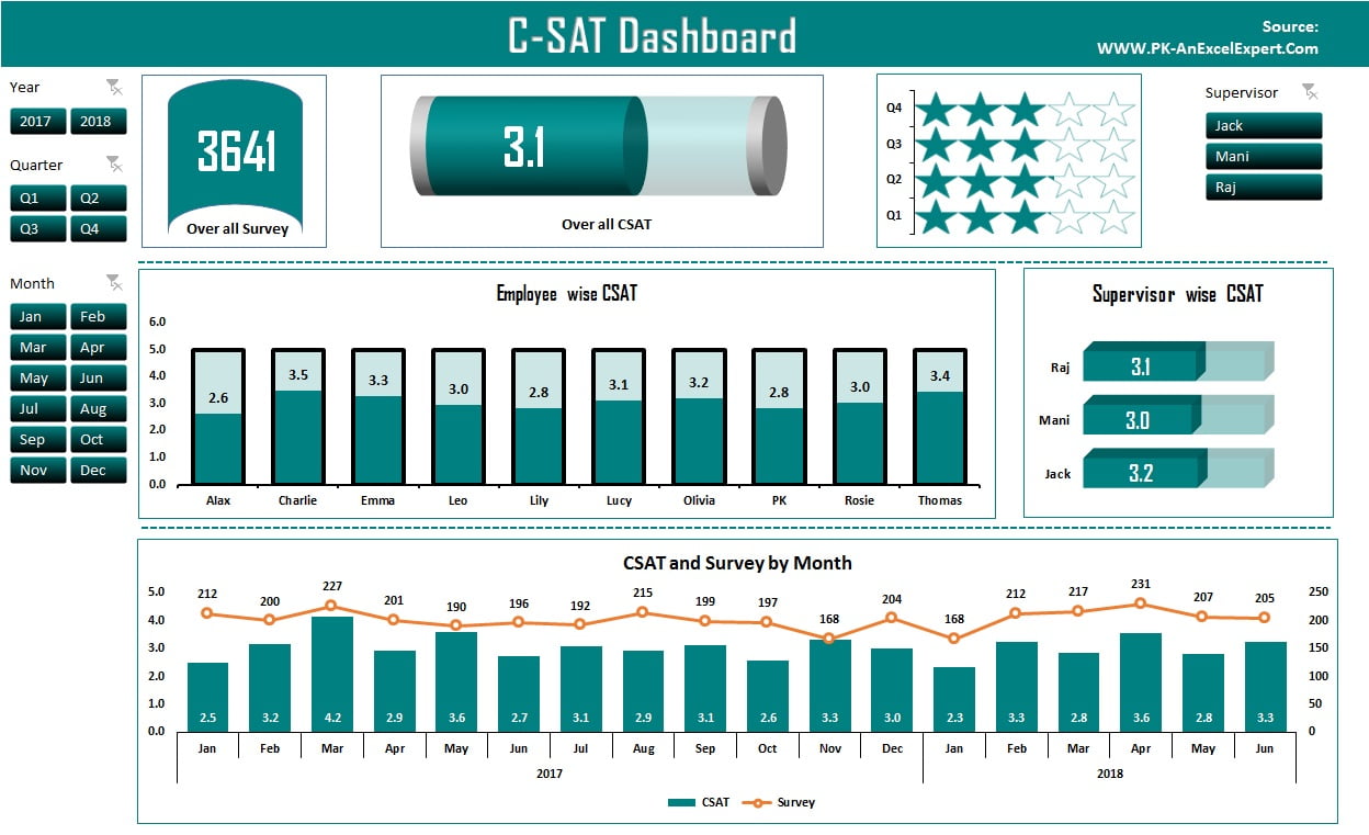
A C-SAT dashboard in Excel shows customer satisfaction, the share of positive survey responses, at overall, quarterly, employee and supervisor level on one page. This C-SAT Dashboard is built from a survey table, four PivotTables and four slicers for Year, Quarter, Month and Supervisor, and presents the numbers in a battery chart, a star rating chart, a filling column chart, a 3-D bar chart and a combo chart. This lesson explains what each section shows, how the pivots and charts are wired and how to load your own survey data.

What the C-SAT Dashboard shows

C-SAT (customer satisfaction score) is satisfied responses divided by total responses, expressed as a percentage. The dashboard answers four questions: what is the overall C-SAT for the selected period, how does it vary by quarter, which employees and supervisors are above or below target, and how do C-SAT and survey volume move month by month. The page is divided into three bands.

Upper band: overall and quarterly C-SAT

A battery chart shows overall C-SAT for the filtered period as a fill level, and a star chart shows each quarter’s C-SAT as a rating out of five. Both are small stacked charts that read a single cell each from the pivot totals, so they respond to every slicer click.

Middle band: employee and supervisor C-SAT

Employee-wise C-SAT appears in a filling column chart, a stacked column where the top segment is the remainder to 100 percent in grey. Supervisor-wise C-SAT is a 3-D bar chart, so individual and team performance are visible together and can be read against the same target line.

Bottom band: monthly trend against volume

A combo chart plots monthly C-SAT as a line on the secondary axis against the number of surveys as columns on the primary axis. This is the most important chart on the page: it shows whether a high score rests on a large sample or on a handful of surveys.

The workbook structure

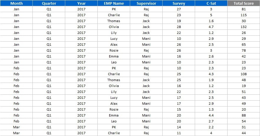
The file follows the three-layer pattern used throughout this course. The Data sheet has one row per survey with Date, Employee, Supervisor and Response, plus helper columns for Year, Quarter and Month derived from the date. The Calculation sheet holds four PivotTables (overall, by quarter, by employee, by supervisor and by month) built on the Data table. The Dashboard sheet holds only the slicers, the charts and the linked labels.

How it is built

Element	Technique	Formula or feature
Year, Quarter, Month helpers	Formulas in the Data table	=YEAR([@Date]), ="Q"&ROUNDUP(MONTH([@Date])/3,0), =TEXT([@Date],"mmm")
Satisfied flag	Helper column	=IF([@Response]="Satisfied",1,0)
C-SAT percentage	PivotTable with Sum of Satisfied and Count of Response	Calculated field =Satisfied/Surveys, or a worksheet cell =SUMIFS(...)/COUNTIFS(...)
Slicers	Insert > Slicer on the first pivot	Report Connections ticked for all pivots
Battery chart	Stacked bar on two cells	Value and =1-value, remainder formatted grey
Star rating	Stacked column, five segments	Quarter C-SAT times 5, split into whole and partial stars
Filling column chart	Stacked column	Employee C-SAT plus =1-C-SAT as the grey top
Supervisor chart	3-D bar chart	Reads the supervisor pivot directly
Trend chart	Combo chart	Columns = surveys, line = C-SAT on the secondary axis

Calculating C-SAT in the PivotTable

The pivot has Sum of Satisfied and Count of Response in the Values area. Add a calculated field with PivotTable Analyze > Fields, Items and Sets > Calculated Field named C-SAT with the formula =Satisfied/Response and format it as a percentage. Because it divides the totals rather than averaging row percentages, every slicer combination stays correct. If you prefer worksheet formulas, =SUMIFS(Data[Satisfied], Data[Month], $B$2)/COUNTIFS(Data[Month], $B$2) gives the same result for a selected month.

Connecting the slicers

Insert the four slicers from the overall pivot, then right-click each slicer, choose Report Connections and tick every PivotTable in the workbook. A slicer that is connected to only one pivot filters one chart and leaves the others unchanged, which is the most common fault in this build. Slicers are covered in detail in Pivot Table chapter 10.

Feeding the charts

Each chart reads a small feed range beside its pivot rather than the pivot itself, using =GETPIVOTDATA or a direct cell reference. The feed range adds the remainder column for the battery and filling charts and multiplies quarterly C-SAT by five for the star chart. When the pivot refreshes, the feed range and the chart follow.

Worked example

Suppose the Data sheet holds these five surveys for January.

Date	Employee	Supervisor	Response	Satisfied
03 Jan	Asha	Rohit	Satisfied	1
05 Jan	Asha	Rohit	Not satisfied	0
09 Jan	Ben	Rohit	Satisfied	1
14 Jan	Ben	Rohit	Satisfied	1
21 Jan	Chloe	Meera	Satisfied	1

With the Month slicer set to Jan, the overall pivot returns Satisfied 4 and Surveys 5, so C-SAT is =4/5 = 80 percent and the battery fills four-fifths. The employee pivot returns Asha 50 percent, Ben 100 percent and Chloe 100 percent. The supervisor pivot returns Rohit 75 percent (3 of 4) and Meera 100 percent (1 of 1). Note that averaging the three employee percentages would give 83 percent, not 80 percent, which is why the calculated field divides totals. The combo chart plots five surveys as a column and 80 percent as the line point for January.

How to use it with your own data

1. Paste your survey rows into the Data table with the same headers: Date, Employee, Supervisor, Response.
2. Check that the Year, Quarter, Month and Satisfied helper columns have filled down (they do automatically in an Excel Table).
3. Go to Data > Refresh All so every PivotTable reads the new rows.
4. Clear all slicers and compare the overall C-SAT with your source report.
5. If your target is not 80 percent, change the target cell that drives the colour thresholds and the target line.

Get the file

The finished C-SAT Dashboard workbook is available as a ready-to-use template: Get the C-SAT Dashboard in Excel. The four videos below show the build from a blank workbook, so you can also rebuild it with your own data.

Watch the video

Four-part build tutorial:

Visit our YouTube channel for more step-by-step dashboard tutorials.

Tips and common mistakes

• Divide totals, never average percentages. C-SAT is satisfied divided by surveys for the whole selection; an average of employee scores weights a two-survey agent the same as a hundred-survey agent.
• Show the survey count beside the score. A 100 percent C-SAT from two surveys is not a result. The combo chart exists for this reason.
• Connect every slicer to every pivot. Use Report Connections after adding any new PivotTable.
• Use real dates. Text dates break the Year, Quarter and Month helpers and put the slicers out of order.
• Keep the raw data as an Excel Table. New survey rows are then included on refresh without changing the pivot source.
• Use one target across the page. Colour the battery, the employee bars and the supervisor bars against the same cell.
• Refresh at the survey cadence. Daily feeds need a daily refresh; a weekly review can use a weekly one.

Errors and how to fix them

Symptom	Cause	Fix
One chart ignores a slicer	Slicer not connected to that chart’s pivot	Right-click the slicer, Report Connections, tick the pivot
C-SAT above 100 percent	Satisfied column holds counts or text instead of 1 and 0	Recreate the helper as =IF([@Response]="Satisfied",1,0)
Months out of order in the slicer	Month helper is text sorted alphabetically	Sort the slicer by a custom list, or use a month number helper
Battery chart empty after refresh	Feed cell references moved when the pivot grew	Point the feed cell at the pivot with GETPIVOTDATA
New surveys missing	Data range is fixed, not a Table	Press Ctrl+T on the data and change the pivot source to the Table name

Practice exercise

1. Add a Channel column (Phone, Email, Chat) to the survey data and build a fifth slicer connected to all pivots.
2. Replace the Satisfied or Not response with a 1 to 5 rating and rebuild the helper so ratings of 4 and 5 count as satisfied.
3. Add a KPI card that shows the number of surveys in the current selection using GETPIVOTDATA.
4. Add a conditional formatting rule to the employee feed range that flags any employee under 70 percent with fewer than ten surveys.
5. Rebuild the monthly combo chart with the target as a third series drawn as a dashed line.

Key takeaways

• C-SAT is satisfied responses divided by total responses; calculate it from totals in the pivot.
• One survey table, four pivots and four slicers drive every chart on the page.
• Report Connections is what makes one slicer filter every chart.
• Battery, star and filling column charts are stacked charts with a grey remainder series.
• Always plot volume next to the score so readers can judge the sample size.

Related lessons

• Excel Dashboards course hub
• Prepare data for an Excel dashboard
• KPI cards and Form Controls in Excel
• Performance Dashboard in Excel
• Outbound Dashboard in Excel
• Slicers in a PivotTable
• COUNTIFS function
• Microsoft Support: COUNTIFS function

Frequently asked questions

How is C-SAT calculated in the dashboard?

As the number of satisfied responses divided by the number of surveys for the filtered period. The PivotTable holds a calculated field that divides the two totals, so every slicer combination, from one employee in one month to the whole year, returns the correct percentage rather than an average of averages.

Can I use a 1 to 5 rating scale instead of satisfied or not?

Yes. Add a helper column that returns 1 when the rating is 4 or 5 and 0 otherwise, and the rest of the dashboard works unchanged. Alternatively change the calculated field to average rating and rescale the battery and star charts to a maximum of 5.

Why does one chart not respond to the slicer?

The slicer is not connected to that chart’s PivotTable. Right-click the slicer, open Report Connections and tick every PivotTable. Repeat for each slicer after you add a new pivot to the workbook.

How often should I update the C-SAT dashboard?

Match the survey feed. If responses arrive daily, paste the new rows and refresh daily; for a monthly review a monthly refresh is enough. Keeping the data as an Excel Table means the refresh is a single Refresh All click.

What is a good C-SAT score?

Most support teams treat 80 percent as the floor and 90 percent or more as strong, but the right target depends on your industry and question wording. Set the target cell on the dashboard to your own benchmark and read every chart against it.

Want the finished version? Ready-made Excel dashboards, trackers and VBA systems are available at NextGenTemplates.com.