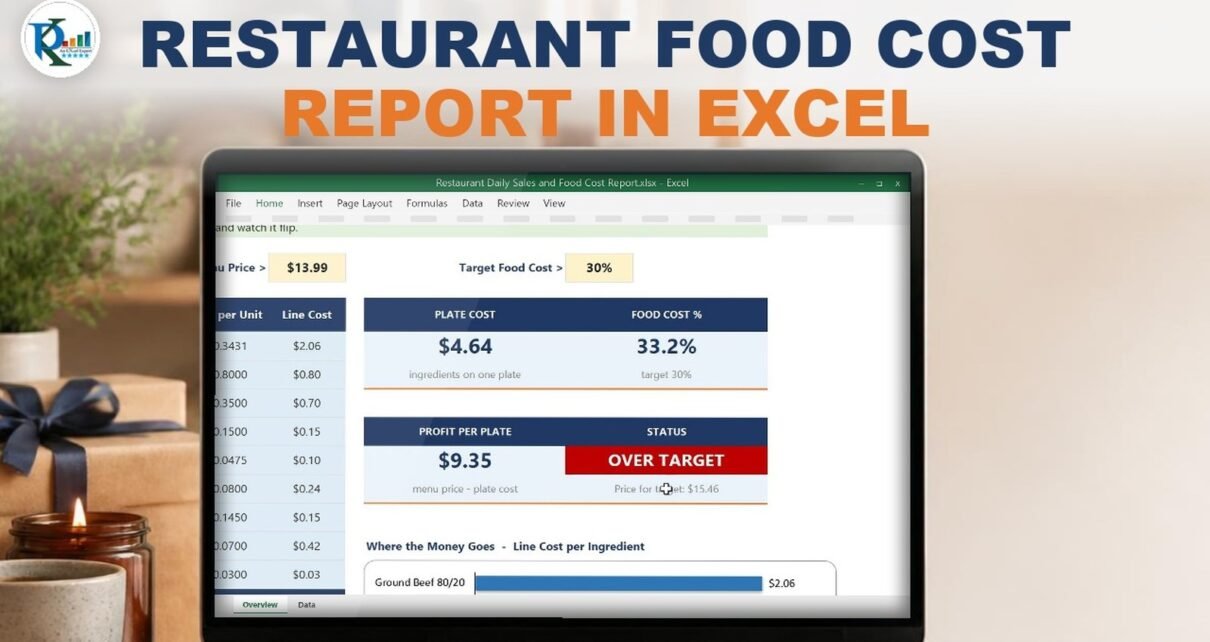
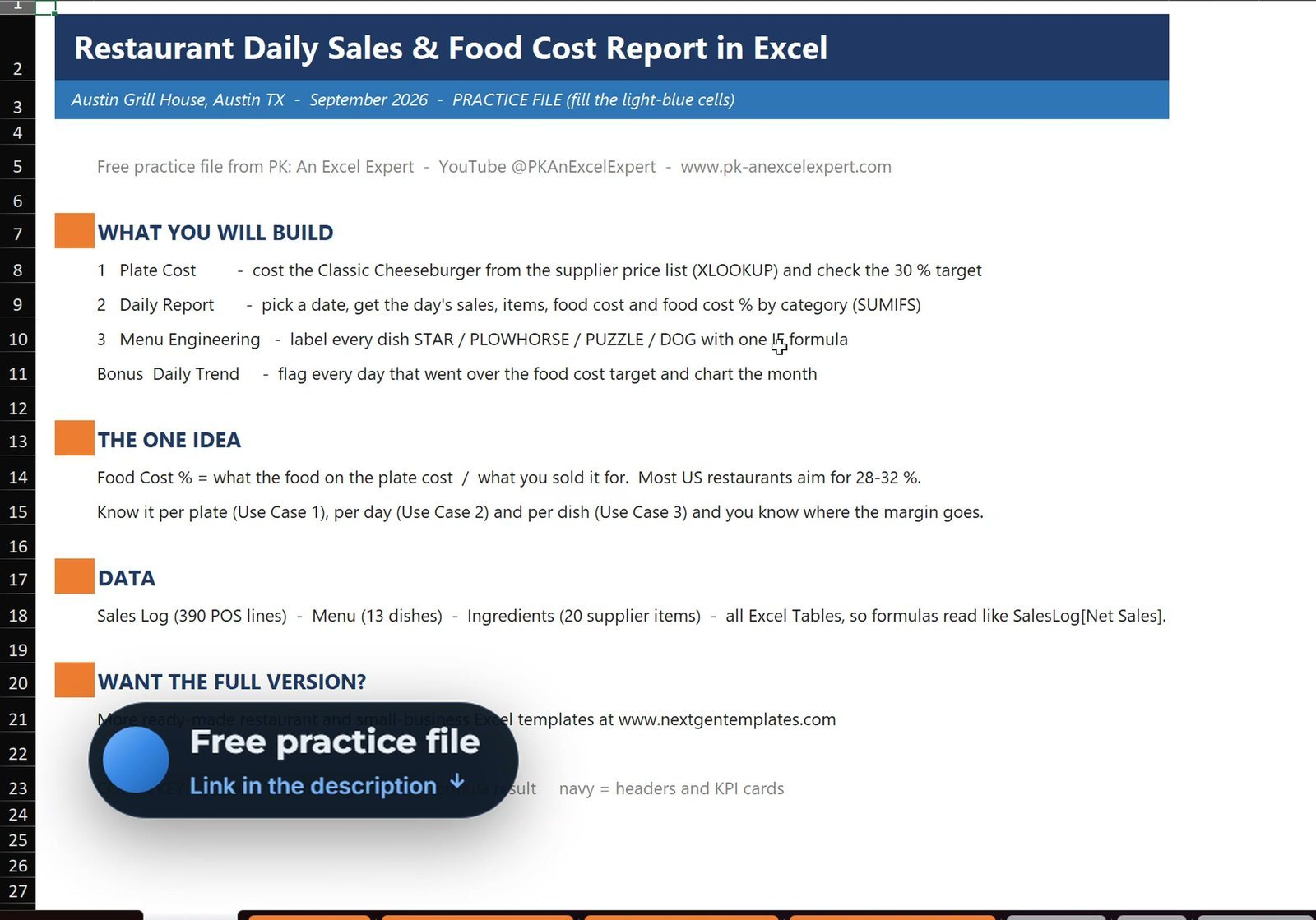
Is your best-selling burger quietly eating your margin? This free food cost calculator Excel file answers that for Austin Grill House, a restaurant in Austin, Texas, with September’s 390 point-of-sale lines, 13 dishes and 20 supplier items. You build it in three parts plus a bonus: the plate cost of one dish with XLOOKUP, a daily sales and food cost report driven by one drop-down and SUMIFS, a menu engineering matrix that labels every dish STAR, PLOWHORSE, PUZZLE or DOG, and a daily trend that flags every day over the 30% food cost target. The surprise: the Classic Cheeseburger is the top profit dish of the month, yet it runs at 33.2% food cost.
⬇️ Download the Free Practice File
Practice + Solution workbooks, Austin Grill House data (390 POS lines, 13 dishes, 20 ingredients) · .zip · Microsoft Excel
Watch the Video Tutorial
Video Overview
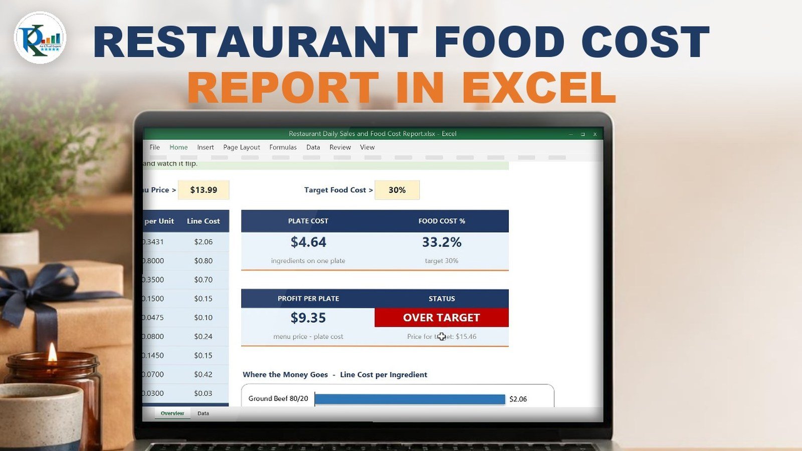
The 10-minute video works in the free practice workbook from start to finish. Part one costs the Classic Cheeseburger line by line: an XLOOKUP pulls each ingredient’s cost per unit from the Ingredients table, a simple multiplication gives the line cost, and SUM gives the plate cost of $4.64 – 33.2% of the $13.99 menu price. Changing the price shows exactly when the badge turns green. Part two turns the 390-line sales log into a one-click daily report: a Data Validation date list, IF + SUMIFS for sales, items and food cost, a status badge and a category breakdown with a two-condition SUMIFS. Part three scores all 13 dishes with menu engineering, and the bonus colours every day that blew the target with a conditional formatting formula.
What This Food Cost Calculator Excel File Does
- Plate cost – cost of one dish from its recipe, the food cost %, profit per plate and the price that hits your target.
- Daily sales report – pick any day and see net sales, items sold, food cost, food cost % and a green or red status badge, with the breakdown by category.
- Menu engineering – units sold, profit per plate and total profit per dish, with each dish classed against the menu averages.
- Daily trend (bonus) – food cost % for all 30 days, every day over target in red, and a line chart against the dashed 30% target.
The Practice Data
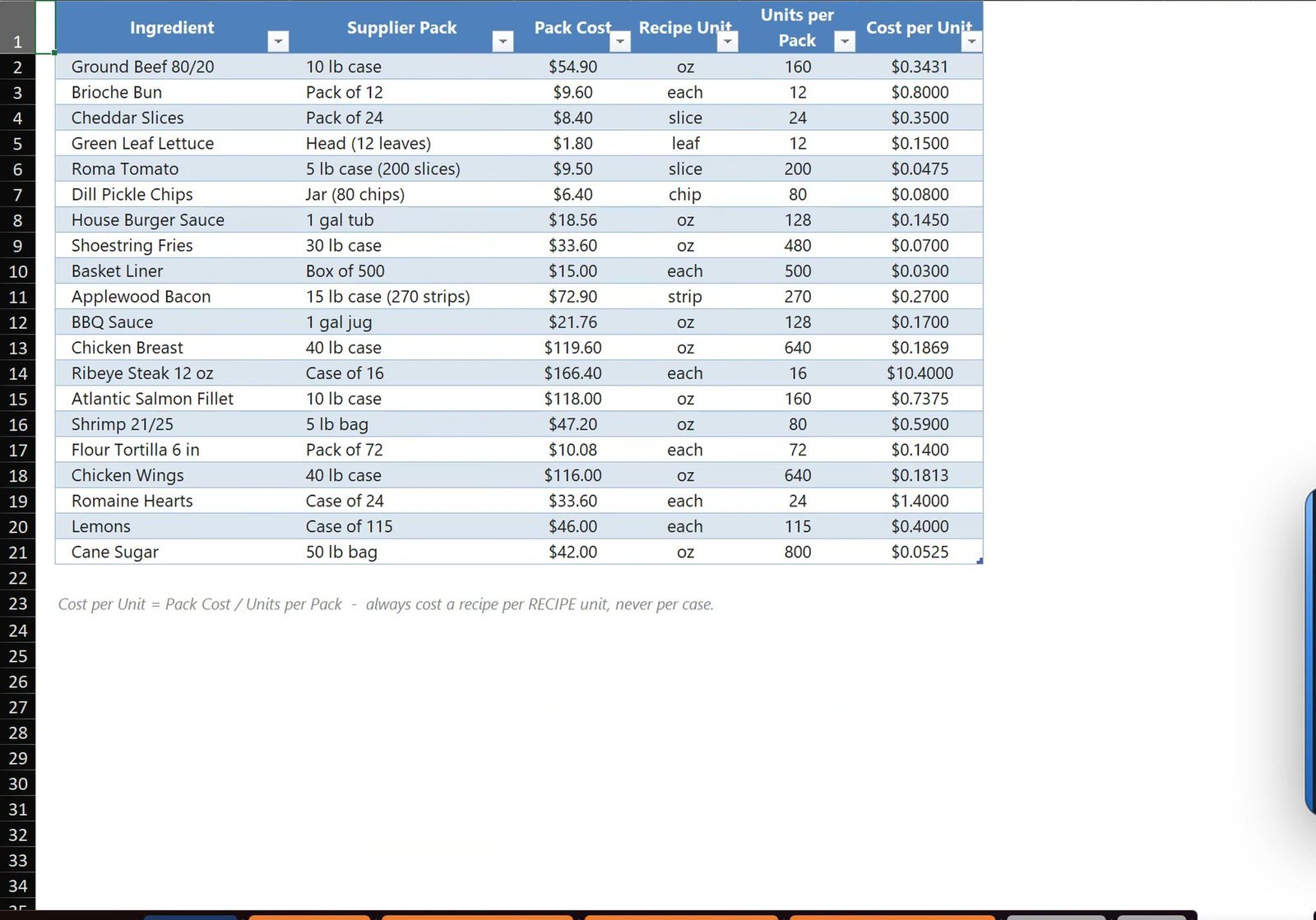
All three data sheets are Excel Tables: Sales Log (390 POS lines with date, item, category, quantity sold, net sales and food cost), Menu (13 dishes with their category and menu price) and Ingredients (20 supplier items with pack cost, units per pack and cost per unit). The one idea behind the whole file: food cost % = what the food on the plate cost / what you sold it for, and the target is 30%.
Part 1: Plate Cost With XLOOKUP
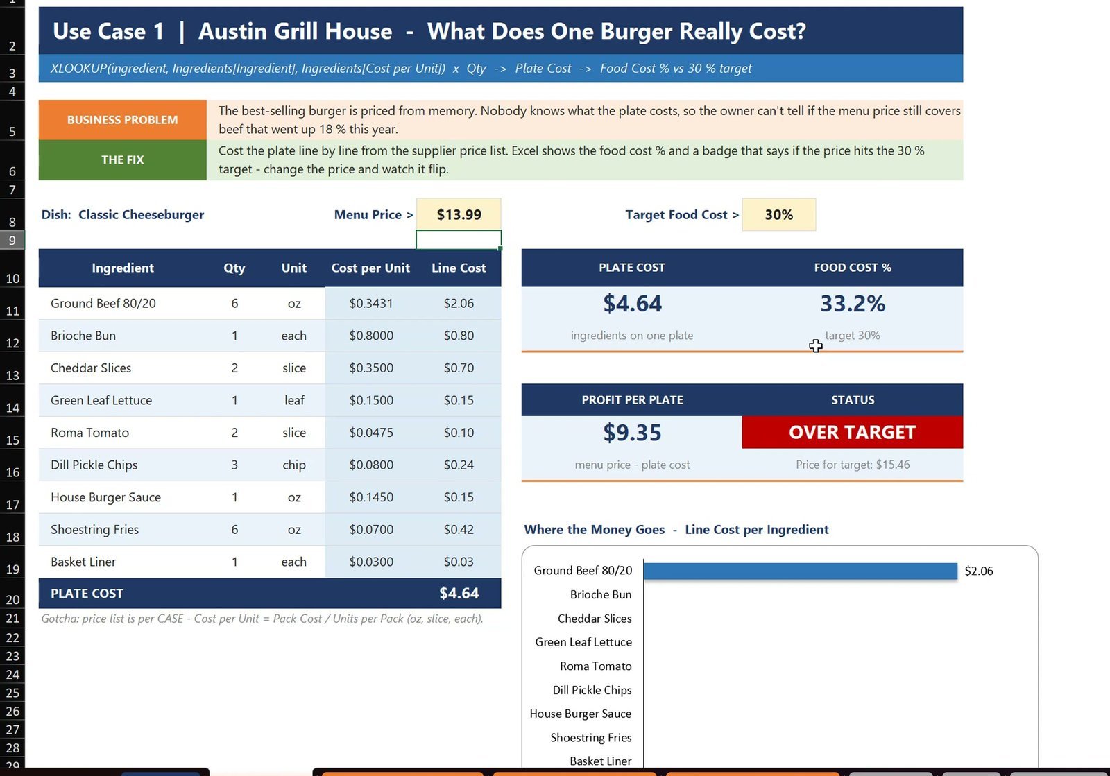
Open the 1. Plate Cost sheet. The Classic Cheeseburger sells for $13.99 and has nine ingredients with their quantities. Nobody knows what one plate really costs – so cost it line by line.
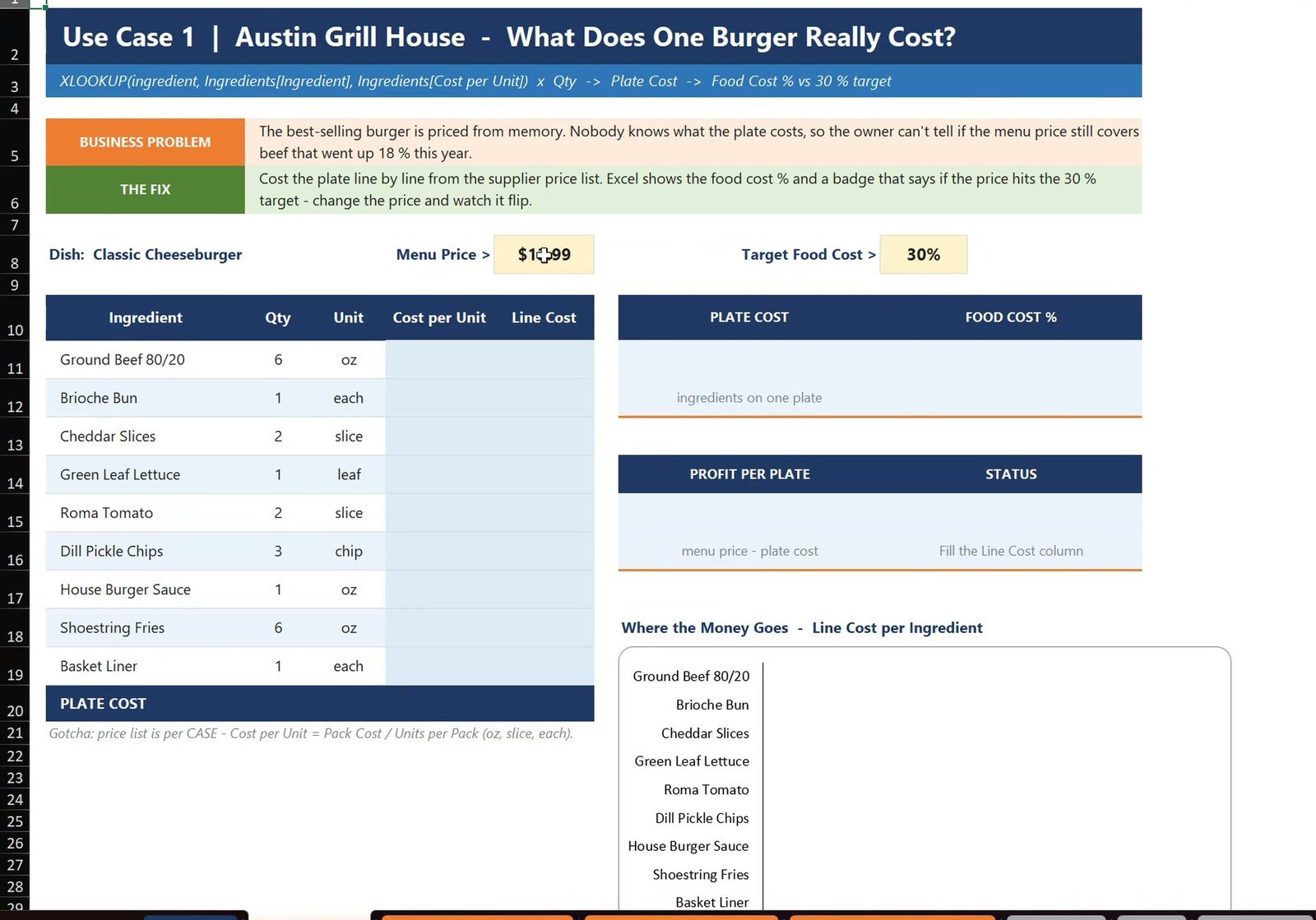
- In E11, look up the cost per unit of the ingredient in B11. Click the Ingredients tab and select the columns with Ctrl+Shift+Down – Excel writes the structured references for you:
=XLOOKUP(B11,Ingredients[Ingredient],Ingredients[Cost per Unit])- In F11, the line cost is quantity times cost per unit:
=C11*E11. Select E11:F19 and press Ctrl+D to fill down. - In F20, add up the lines:
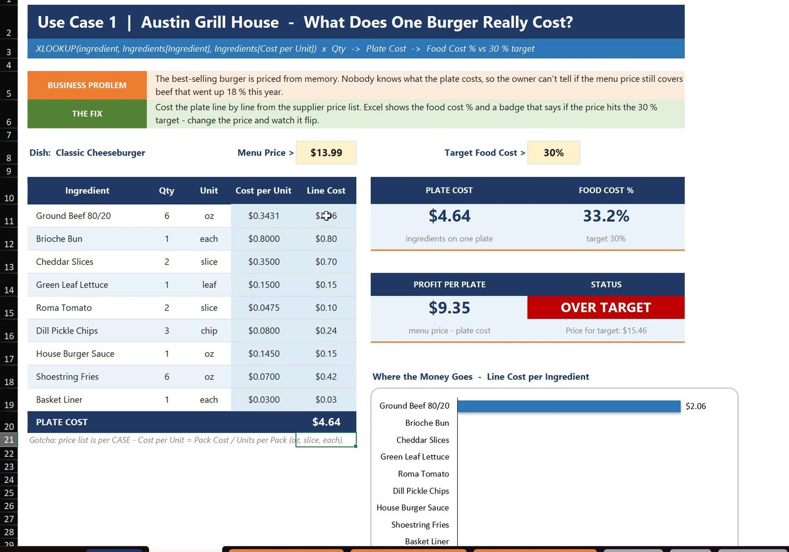
=SUM(F11:F19). The plate cost is $4.64.
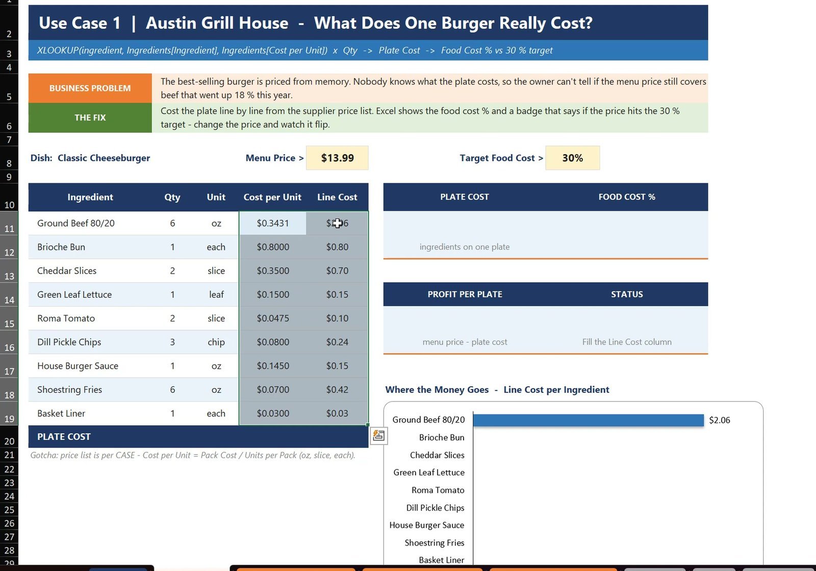
Gotcha: the supplier sells beef by the case, so the cost per unit is the pack cost divided by the units per pack – $54.90 / 160 oz = $0.3431 per ounce. Use the case price by mistake and the plate cost is wildly wrong.
The cards fill themselves: food cost 33.2%, profit per plate $9.35, and the status says OVER TARGET in red. The “Where the Money Goes” chart shows the beef alone is $2.06 – about 44% of the plate.
Find the Menu Price for a 30% Food Cost
The card shows the price for the target: $4.64 / 30% = $15.46. Type 14.99 in F8: 30.9%, still over. Type 15.99: 29.0%, and the badge turns green. (Put 13.99 back – Part 3 uses the real menu price.)
Part 2: Restaurant Daily Sales Report With One Drop-Down
Every morning the manager adds up yesterday by hand from 390 POS lines a month. The 2. Daily Sales Report sheet does it from one date drop-down.
Step 1: The Date Drop-Down
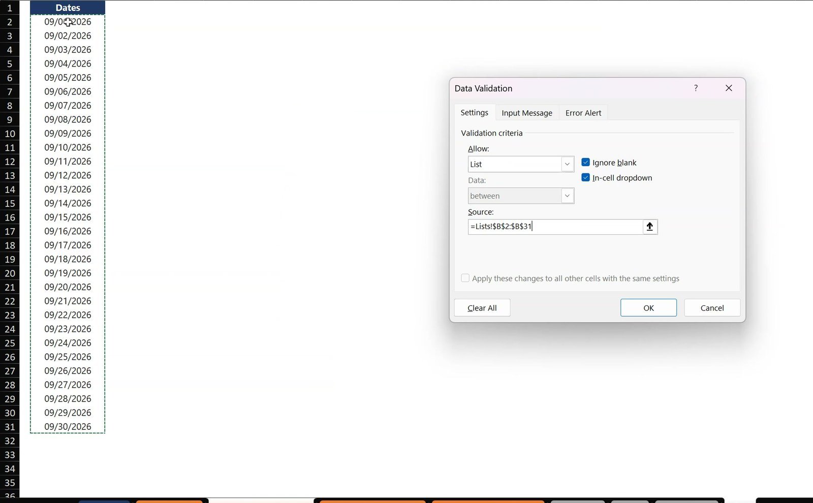
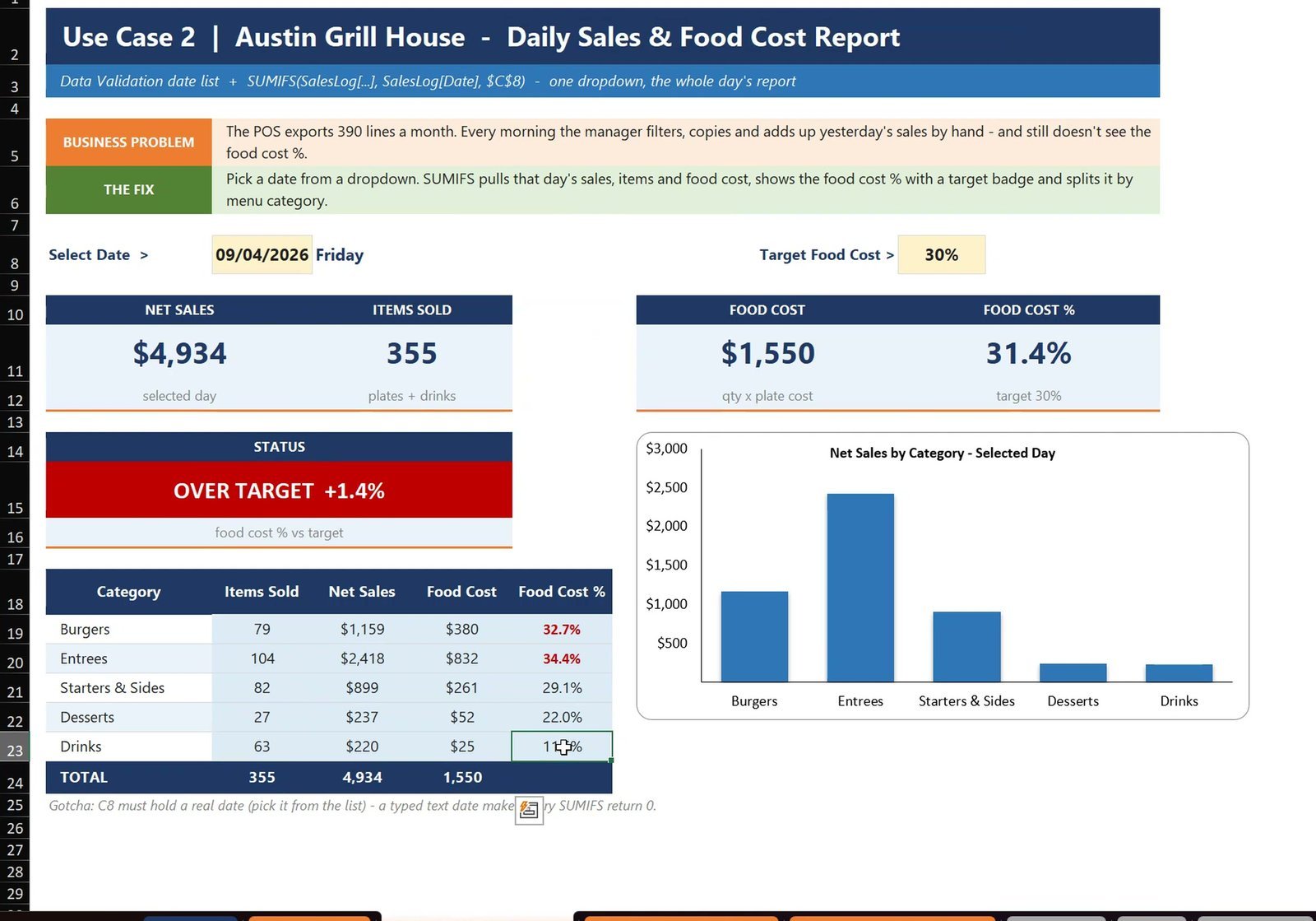
Click C8, go to Data > Data Validation, choose List and set the source to the date list on the Lists sheet (=Lists!$B$2:$B$31). Pick 09/04/2026, a Friday.
Step 2: Sales, Items and Food Cost With IF + SUMIFS
The IF guard keeps the cell empty until a date is picked:
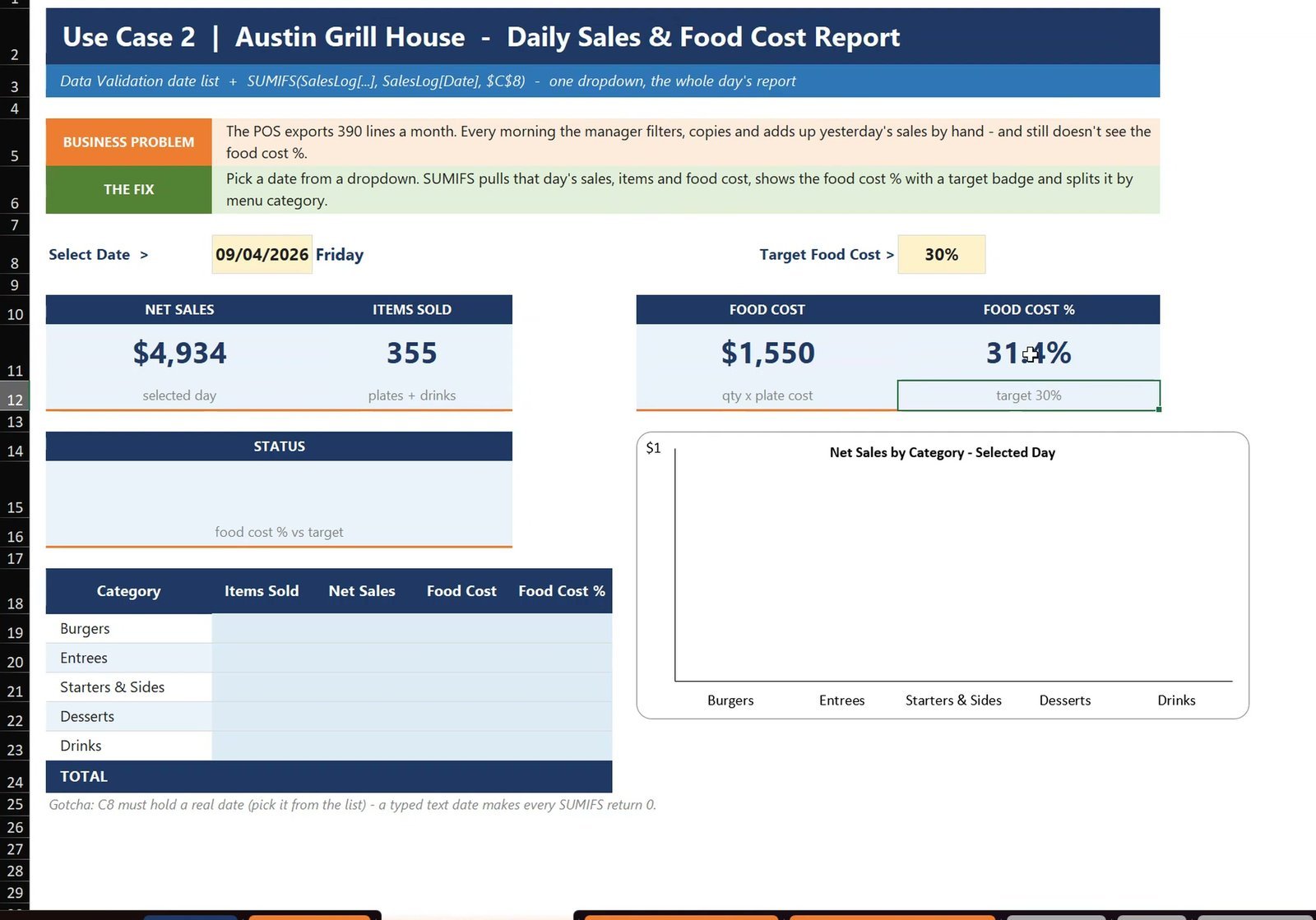
=IF($C$8="","",SUMIFS(SalesLog[Net Sales],SalesLog[Date],$C$8))That gives $4,934 of net sales. The same formula with the Qty Sold column gives 355 items in D11, and with the Food Cost column $1,550 in H11.
Step 3: Daily Food Cost % and the Status Badge
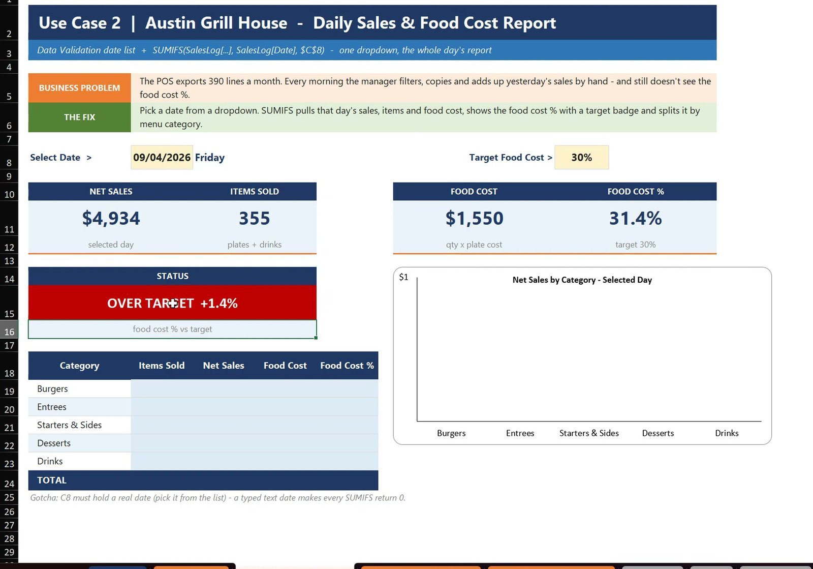
=IF(OR($C$8="",N(B11)=0),"",H11/B11)K11 shows 31.4%. The badge in B15 compares it with the target in K8:
=IF(OR($C$8="",K11=""),"",IF(K11<=$K$8,"ON TARGET","OVER TARGET +"&TEXT(K11-$K$8,"0.0%")))Friday is OVER TARGET +1.4%, in red.
Step 4: Food Cost by Category (SUMIFS With Two Conditions)
Which category drives it? Add a second condition – the date is C8 and the category is B19, with only the column locked (press F4 three times):
=IF($C$8="","",SUMIFS(SalesLog[Net Sales],SalesLog[Date],$C$8,SalesLog[Category],$B19))Fill C19:F23 down with Ctrl+D and add the total row. Friday by category: Entrees 34.4%, Burgers 32.7%, Starters & Sides 29.1%, Desserts 22.0% and Drinks 11.5% – so Entrees and Burgers push Friday over target.
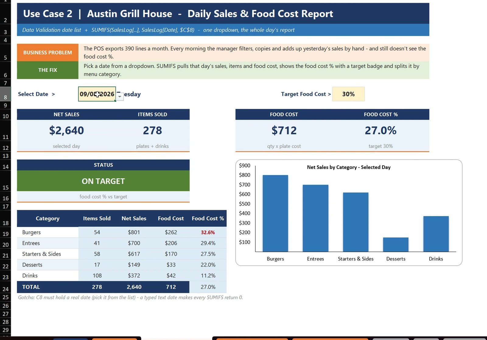
Now pick 09/08/2026, a Tuesday: $2,640 of sales, 27.0%, ON TARGET. Gotcha: C8 must hold a real date. A typed text date makes every SUMIFS return 0.
Part 3: Menu Engineering Matrix in Excel
Popular is not the same as profitable, so the 3. Menu Engineering sheet scores every dish on both.
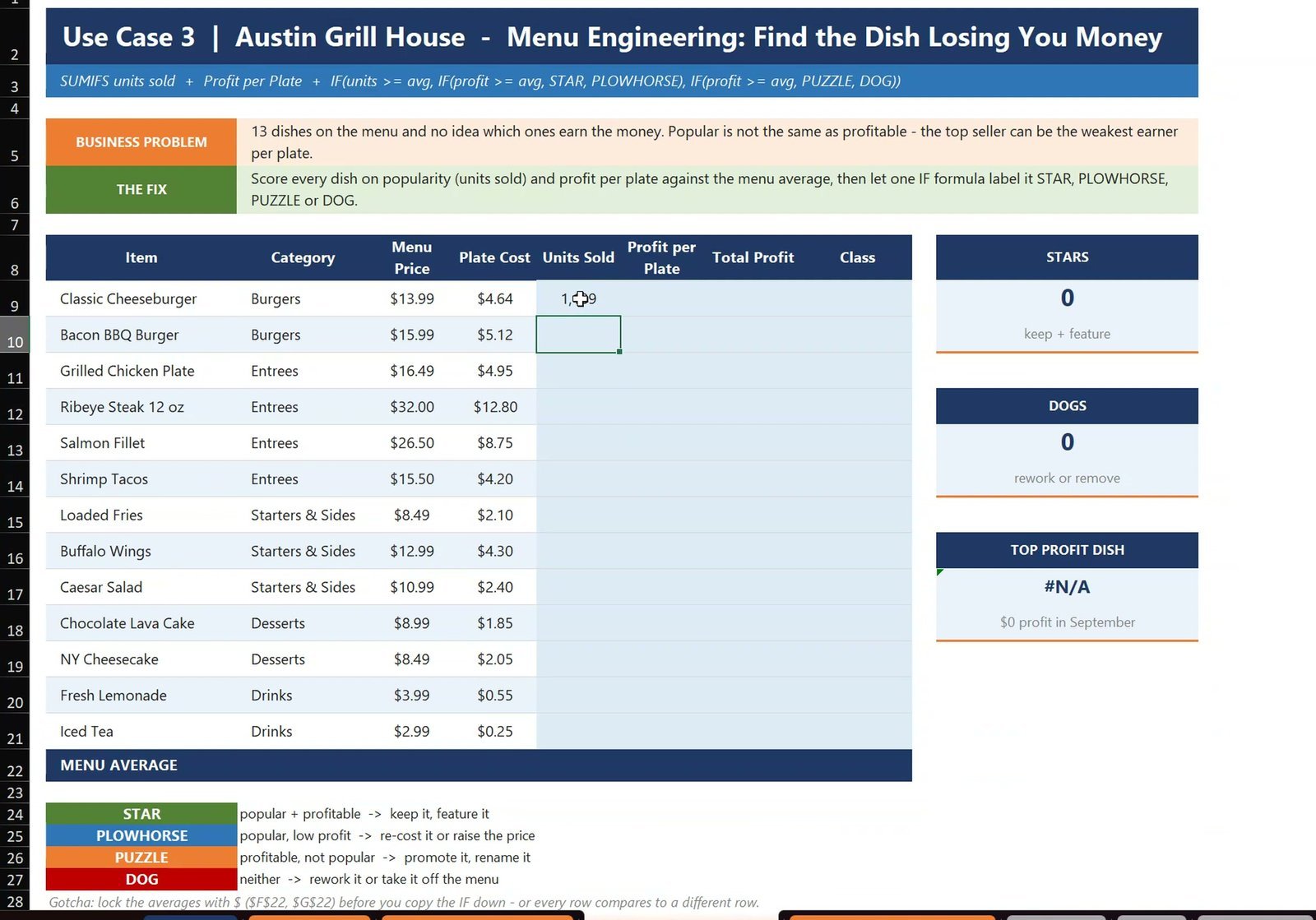
- Units sold per dish in F9:
=SUMIFS(SalesLog[Qty Sold],SalesLog[Item],B9)– 1,189 cheeseburgers in September. - Profit per plate in G9:
=D9-E9(menu price minus plate cost), and total profit in H9:=F9*G9. Fill F9:H21 down. - Averages in row 22:
=AVERAGE(F9:F21)= 712 units, and $9.50 profit per plate in G22.
STAR, PLOWHORSE, PUZZLE or DOG With One Nested IF
=IF(F9>=$F$22,IF(G9>=$G$22,"STAR","PLOWHORSE"),IF(G9>=$G$22,"PUZZLE","DOG"))Double-click the fill handle. Lock the averages with $ first, or every row compares to a different cell.
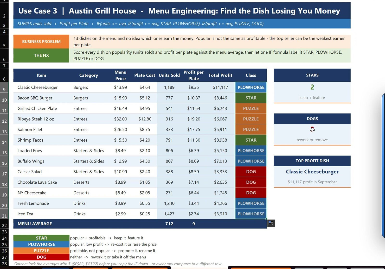
The result: STAR – Bacon BBQ Burger and Shrimp Tacos. PUZZLE – Grilled Chicken, Ribeye and Salmon. DOG – Caesar Salad, Lava Cake and NY Cheesecake. Everything else is a PLOWHORSE.
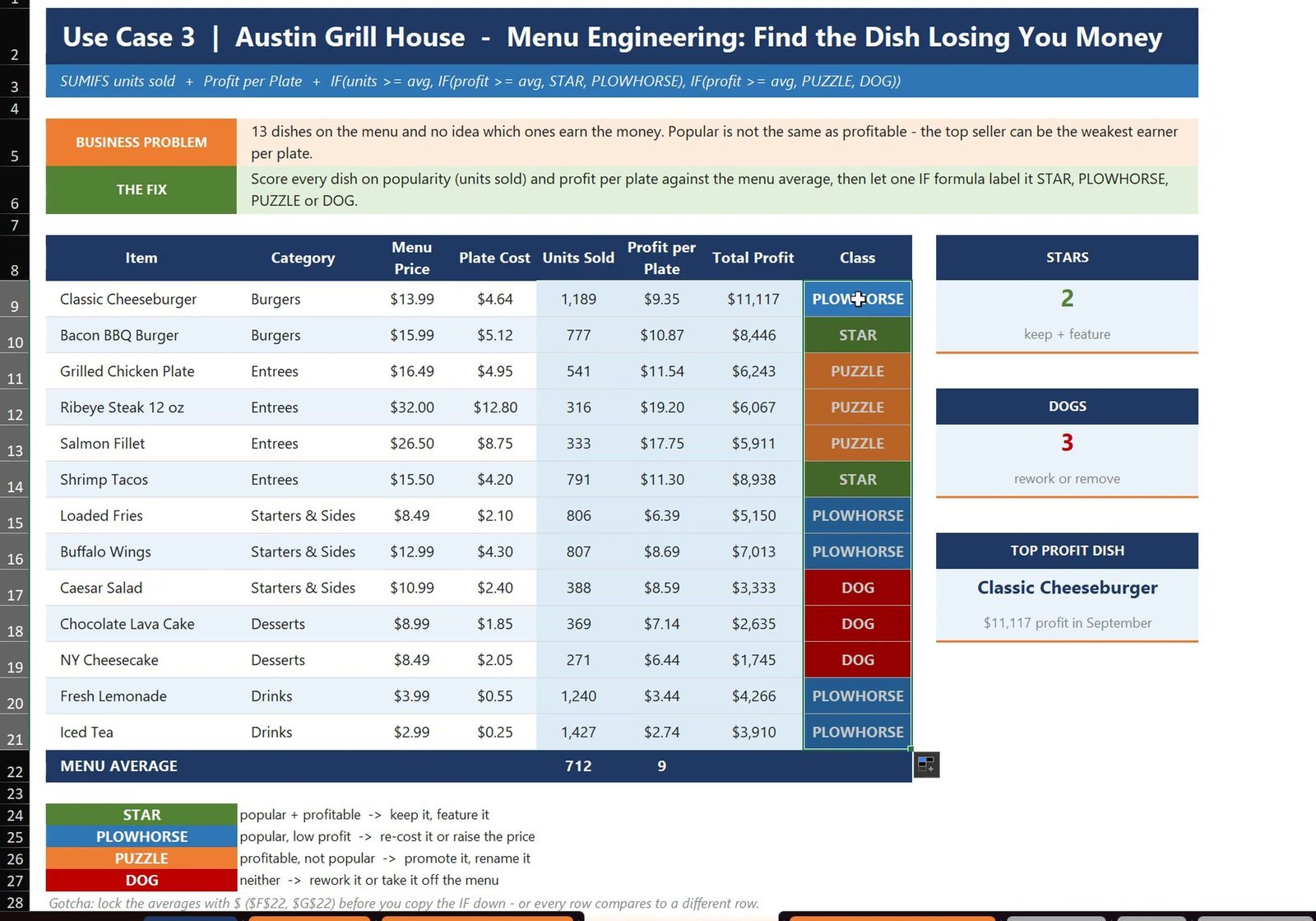
The top profit dish is the Classic Cheeseburger with $11,117 of profit in September – but only because of volume. Per plate it earns $9.35, below the $9.50 average: a plowhorse. That is exactly the price fix from Part 1.
Bonus: Which Days Blew the Food Cost?
On the 4. Bonus – Daily Trend sheet, D9 sums the net sales of the date in B9 with =SUMIFS(SalesLog[Net Sales],SalesLog[Date],$B9), E9 does the same with Food Cost, and F9 divides them: =IF(D9=0,"",E9/D9). Fill D9:F38 down.
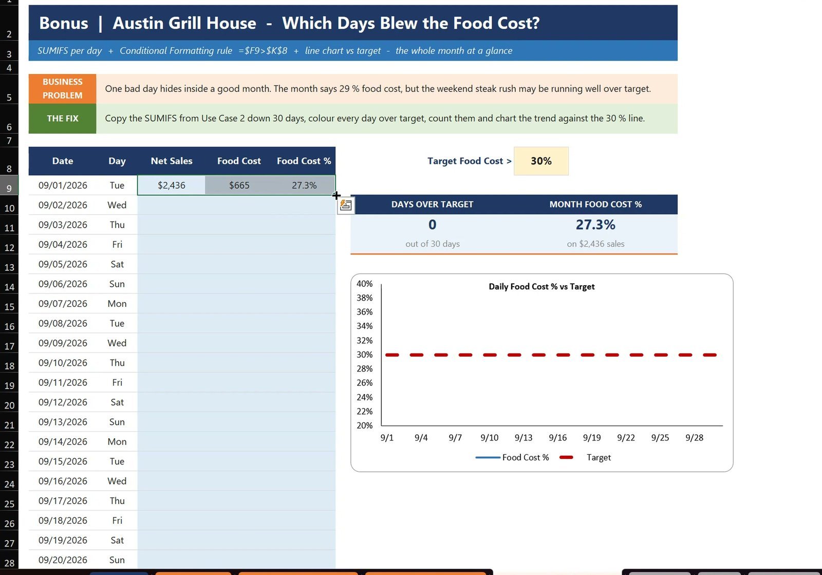
Then select B9:F38, go to Home > Conditional Formatting > New Rule > Use a formula and enter:
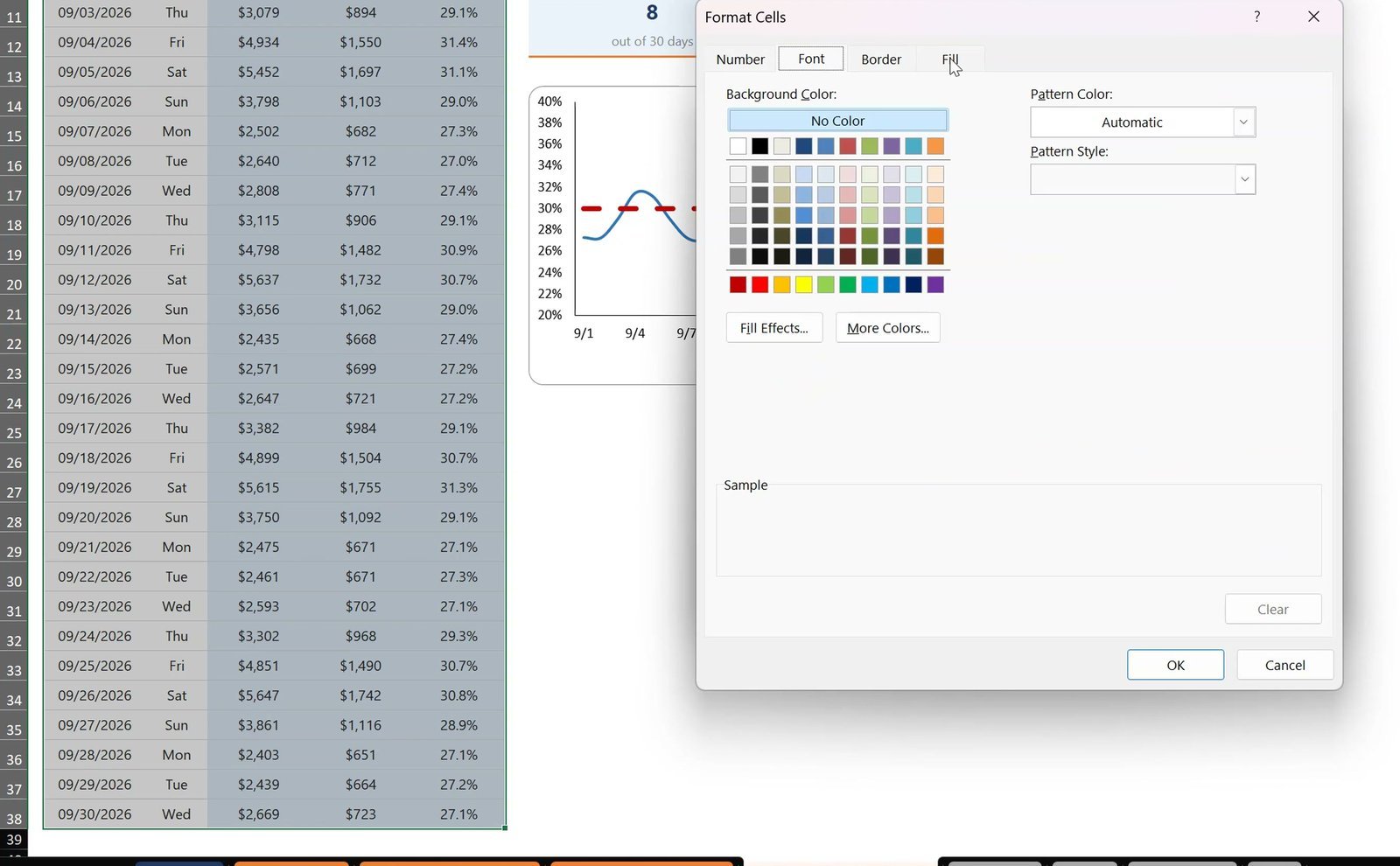
=AND($F9<>"",$F9>$K$8)Click Format, pick a red fill and bold red text, and click OK twice.
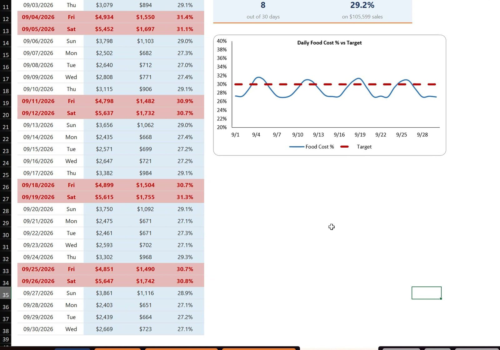
8 days are over target – and every one is a Friday or a Saturday. The month’s food cost is 29.2% on $105,599 of sales. The month looks fine, but every weekend runs over.
Formula Cheat Sheet
| Task | Formula / tool | Result in the file |
|---|---|---|
| Cost per unit of an ingredient | XLOOKUP | Beef $0.3431/oz |
| Plate cost | Qty x cost, then SUM | $4.64 (33.2%) |
| Daily sales / items / food cost | IF + SUMIFS (1 condition) | $4,934 / 355 / $1,550 |
| Food cost by category | SUMIFS (2 conditions) | Entrees 34.4% |
| Menu engineering class | Nested IF vs locked averages | 2 stars, 3 dogs |
| Flag bad days | Conditional formatting formula | 8 days over target |
Tips
- Keep the target in one cell (K8) and point every formula at it – change it once and the whole report follows.
- Use Excel Tables for the sales log so SUMIFS ranges grow automatically when next month’s POS export is pasted in.
- Microsoft’s SUMIFS function reference explains every argument and wildcard.
- Building more business files? Try the billing and invoice system in Excel tutorial, or see the ready-made Food and Beverage Report in Excel and the Restaurants & Food Services KPI Dashboard in Excel.
Want It Ready-Made?
For a complete restaurant report, take a look at the Restaurant P and L Dashboard in Excel on NextGenTemplates.com – it tracks revenue, labor cost, waste and cost of goods sold by branch (read the overview). We also build custom Excel templates and dashboards on demand. To master XLOOKUP, SUMIFS, IF and 97 more formulas step by step, join the Excel + AI Mastery: 100 Essential Formulas course on Next Gen Templates Academy.
Frequently Asked Questions
What is the food cost percentage formula?
Food cost % = cost of the food on the plate / menu price. In this file the Classic Cheeseburger costs $4.64 to make and sells for $13.99, so its food cost is 4.64 / 13.99 = 33.2%. Most restaurants aim for about 28-32%; this report uses a 30% target.
How do I calculate the plate cost of a dish in Excel?
List the ingredients and quantities, pull each ingredient's cost per unit from your supplier table with XLOOKUP, multiply quantity by cost per unit for the line cost, and SUM the lines. The cost per unit must be the pack cost divided by the units per pack – beef at $54.90 per 160 oz case is $0.3431 per ounce.
What menu price hits a 30% food cost?
Divide the plate cost by the target: $4.64 / 0.30 = $15.46. In the video, $14.99 still gives 30.9% (over target) and $15.99 gives 29.0%, which turns the badge green.
Why does my SUMIFS return 0 for a date?
The date cell holds text, not a real Excel date. A typed text date never matches the real dates in the sales log, so every SUMIFS returns zero. Pick the date from a Data Validation list of real dates, as the report does in C8.
What is a menu engineering matrix?
It sorts every dish by popularity (units sold) and profitability (profit per plate) against the menu averages: STAR = popular and profitable, PLOWHORSE = popular but below-average profit, PUZZLE = profitable but slow, DOG = neither.
How do I classify dishes as STAR, PLOWHORSE, PUZZLE or DOG in Excel?
Use one nested IF against the averages with absolute references: =IF(F9>=$F$22,IF(G9>=$G$22,"STAR","PLOWHORSE"),IF(G9>=$G$22,"PUZZLE","DOG")). Lock the averages with $ before filling down, or every row compares to a different cell.
How do I highlight the days that went over the food cost target?
Select the daily table, go to Home > Conditional Formatting > New Rule > Use a formula, and enter =AND($F9<>"",$F9>$K$8), where column F is the daily food cost % and K8 the target. Pick a red fill and bold red text.
Is the practice file free?
Yes. The zip has the practice workbook to follow along and the finished solution workbook. You need Microsoft Excel 365 or Excel 2021 for XLOOKUP.
Download the Practice File
Get the practice workbook to follow along and the finished solution workbook in one zip – free.
⬇️ Download the Free Practice File
Practice + Solution workbooks, Austin Grill House data (390 POS lines, 13 dishes, 20 ingredients) · .zip · Microsoft Excel
About the Author
PK (Priyendra Kumar) runs PK: An Excel Expert and NextGenTemplates.com and has been teaching Excel, VBA and Power BI on YouTube for years. Every step in this tutorial was recorded in the real Microsoft Excel with the files you can download above.
Conclusion
A restaurant food cost report does not need an expensive system. With XLOOKUP for the plate cost, IF + SUMIFS for the daily report, one nested IF for menu engineering and a conditional formatting formula for the trend, you see in seconds which dishes and which days cost you money – and which price fixes it. Download the free file and run it on your own POS export.