Microsoft Excel is a robust and Powerful tool that has established itself for data analysis, record-keeping, and financial modeling. Its utilization has become an indispensable aspect of nearly every field from finance and accounting to marketing and sales. Nevertheless, a lot of features and techniques are there which may not be in your awareness. These tips can markedly enhance your efficiency and productivity. Thus, in this article, we will explain seven excellent tips within Microsoft Excel that can unlock its full potential and help you maximize your output.
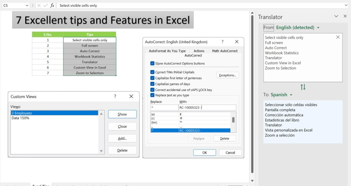
Select Visible Cells Only:
Sometimes, you may want to copy only the visible cells and exclude the hidden cells in your selected range. You can do this quickly by selecting the visible cells only. Below are the steps to do this-
- Step 1: Select the range of cells that you want to copy.
- Step 2: Click on the “Find & Select” button in the “Editing” group on the “Home” tab.
- Step 3: Select the “Go To Special”.
- Step 4: In the “Go To Special” dialog box, select “Visible cells only” and click “OK.”
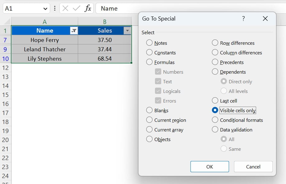
Alternatively, you can use the shortcut key “Alt+;.” This will select only the visible cells in your range. You can copy it easily and paste it without including the hidden cells.
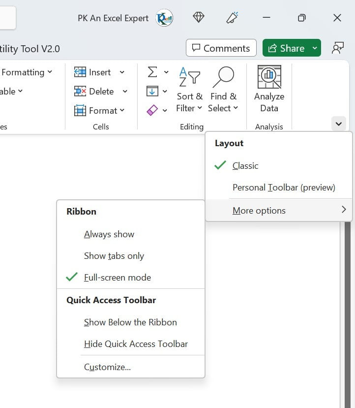
Full Screen:
Excel’s full-screen mode can be handy when you want to focus on a specific worksheet or when you want to hide the ribbon and other distracting elements. You can press the shortcut key “Ctrl+Shift+F1” to activate full-screen mode. Press the same shortcut key again to exit full-screen mode.
Auto Correct:
Excel’s AutoCorrect feature can save a lot of time and effort by automatically correcting common spelling and typing errors. You can also add your own entries to the AutoCorrect list. Below are the steps to do this-
- Step 1: Click on the “File” tab and select “Options” or press shortcut key Alt+T+O.
- Step 2: In the “Excel Options” window, select “Proofing” from the list on the left side.
- Step 3: Click on the “AutoCorrect Options” button.
- Step 4: In the “AutoCorrect” window, you can add your own entries by typing the incorrect spelling. or phrase in the “Replace” box and the correct spelling or phrase in the “With” box. Click “Add” to save the entry.
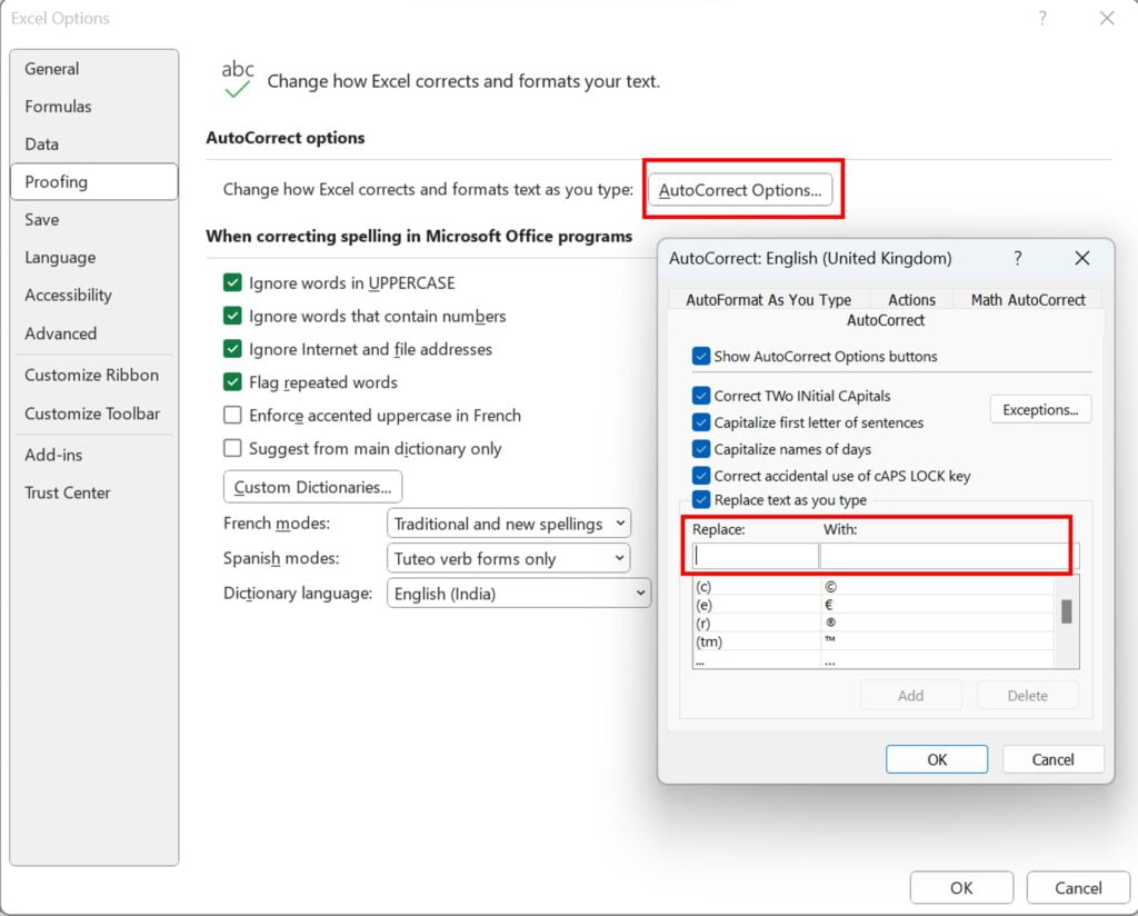
Now, every time you type the incorrect spelling or phrase, Excel will automatically correct it to the correct spelling or phrase.
Workbook Statistics:
Excel’s “Workbook Statistics” feature provides useful information about your workbook like – number of sheets, cells, formulas, and objects.
Follow the below steps to see it-
- Step 1: Go to the “Review” tab.
- Step 2: Click on the “Workbook Statistics” button in the “Proofing” group.
- Step 3: In the “Workbook Statistics” popup, you can see information about your workbook like- the number of sheets, cells, formulas, and objects.
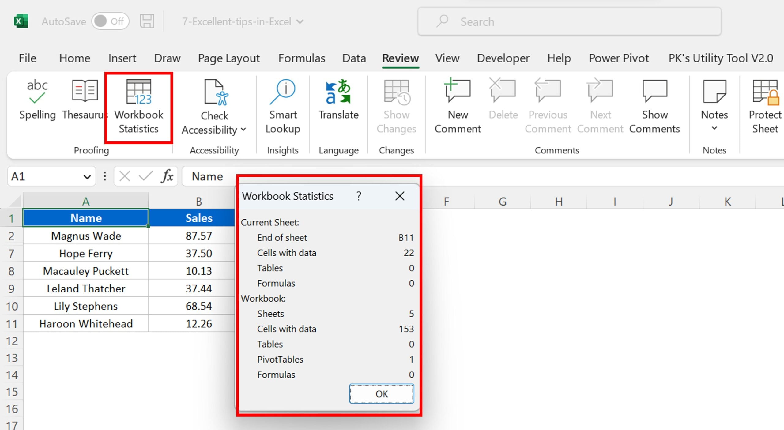
Alternatively, you can use the shortcut key “Alt+R+B” or “Ctrl+Shift+G” to see the “Workbook Statistics”.
Translator:
Excel’s “Translate” feature allows you to translate text from one language to another. You can do this directly inside of your worksheet. This is very useful when you’re working with international data or communicating with clients and colleagues who speak different languages.
Below are the steps to use it-
- Step 1: Select the range of cells that you want to translate.
- Step 2: Click on the “Review” tab on the ribbon.
- Step 3: Click on the “Translate” button in the “Language” group.
- Step 4: In the “Translation” pane, select the desired language for translation.
- Step 5: Click on the “Translate” button.
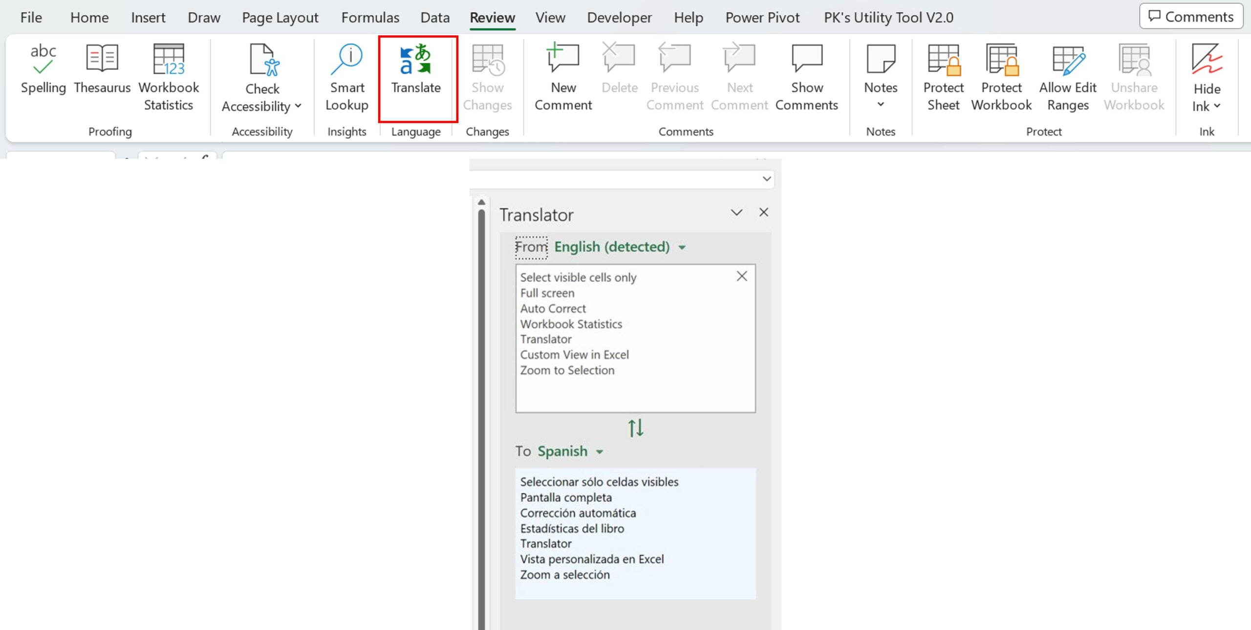
Alternatively, you can use the shortcut keys “Shift+Alt+F7” or “Alt+R+L” to access this feature.
Custom View:
You can save the different views in Excel using Custom View feature. In the custom view, you can save hidden or visible rows or columns or even filter selection. for example, if view-1 you can put the filter for any value and in the view-2 you can put the filter for other value. Custom view works with Print settings also like- headers and footers, margins or print area setting etc.
Follow the below are the steps to create the custom view in Excel –
- Step 1: Click on the “View” tab.
- Step 2: Click on the “Custom Views”.
- Step 3: In the “Custom Views” popup, click on the “Add” button.
- Step 4: In the “Add View” popup just add your custom view name.
- Step 5: Click “OK” to save your custom view.
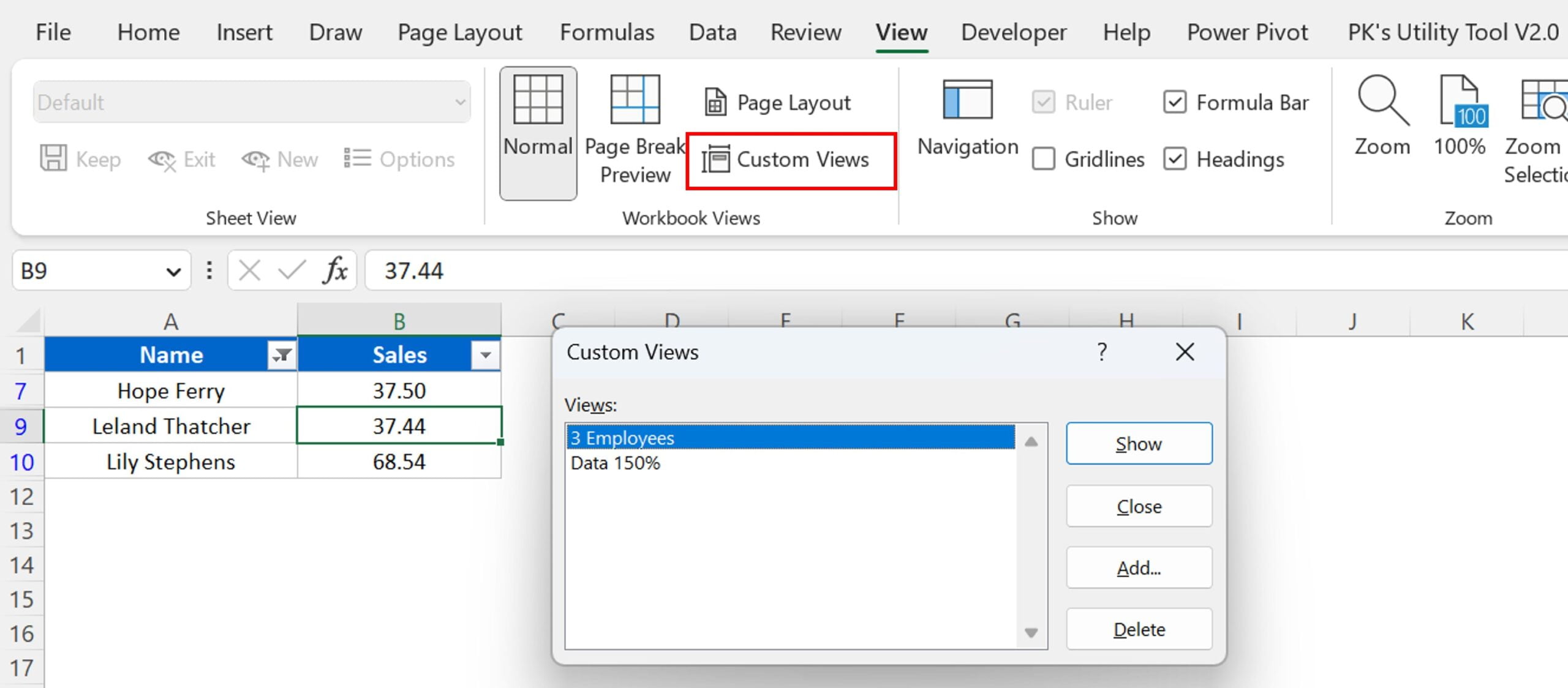
Finally, you can switch between different views by selecting the desired custom view from the “Custom Views” dialog box. Alternatively, you can use the shortcut key “Alt+W+C” to access this feature.
Zoom to Selection:
Zoom to Selection is a useful feature in Excel. It helps to focus on the selected range. It is useful when you have a lot of data and font size is small. To read the data quickly, you can select the desire range and click on zoom to Selection.
Below are the steps to use the Zoom to selection in excel-
- Step 1: Select the range of cells that you want to zoom in on.
- Step 2: Click on the “View” tab on the ribbon.
- Step 3: Click on the “Zoom to Selection” button in the “Zoom” group.
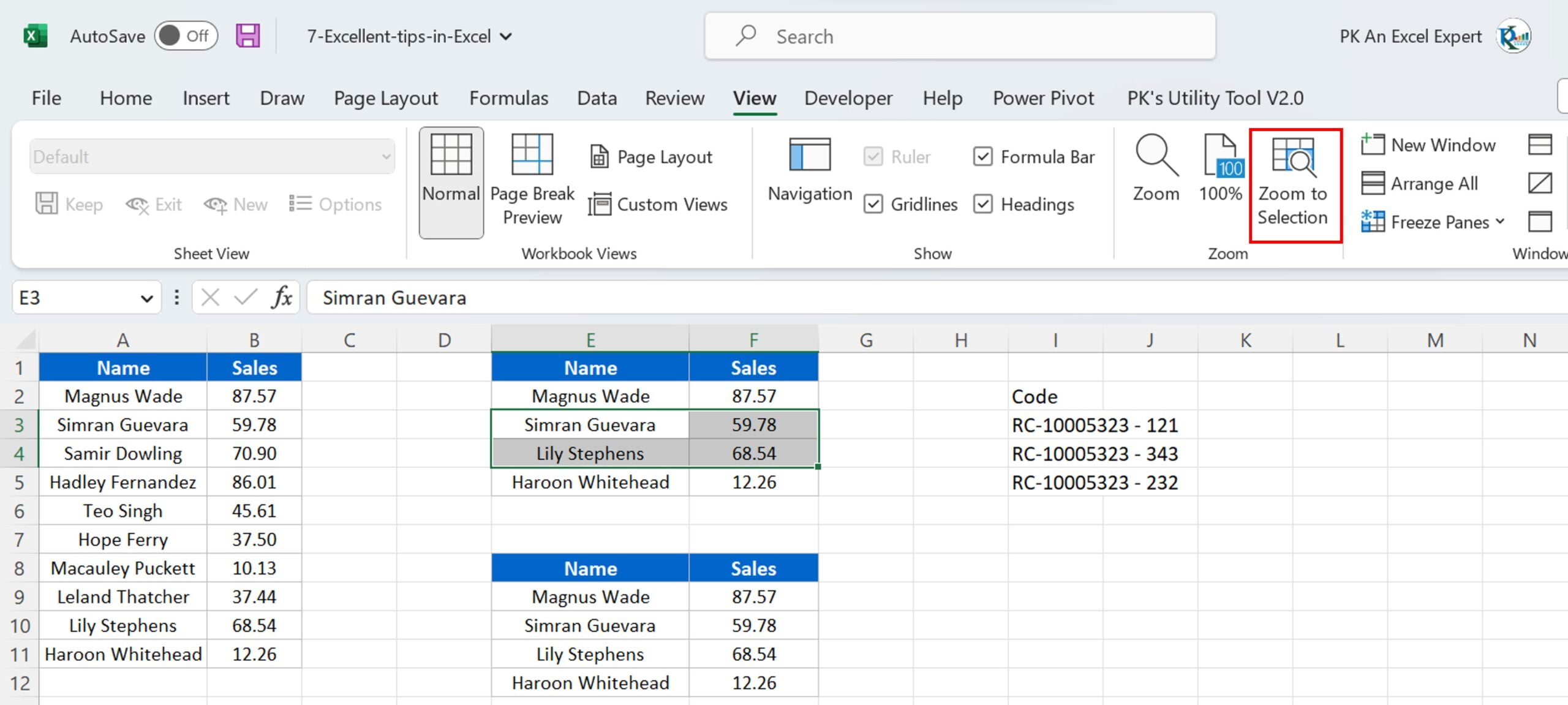
Zoom to Selection
Alternatively, you can also use the shortcut key “Alt+W+G” to use Zoom to select ion in Excel. To return to the original zoom level, press the shortcut key “Alt+W+J.”
Conclusion:
In conclusion, above given seven tips and features can help you work more efficiently and productively in Microsoft Excel. Whether you’re a beginner or an experienced user, these features can save you time and effort and make your work more enjoyable. So, try them out and see how they can help you improve your Excel skills.
Visit our YouTube channel to learn step-by-step video tutorials
Watch the step-by-step video tutorial:
Click here to download the practice file
Visit our YouTube channel to learn step-by-step video tutorials