Excel isn’t just a tool; it’s a canvas for data artists like you. Today, let’s add a splash of interactivity and color to that canvas. We’re diving into a super cool feature—dynamic conditional formatting with a form control checkbox. This isn’t just about making your spreadsheet look pretty; it’s about bringing your data to life, making it tell stories in vivid color. So, grab your data brush; we’re about to paint some magic on the Excel canvas.
Step into the World of Dynamic Data Visualization
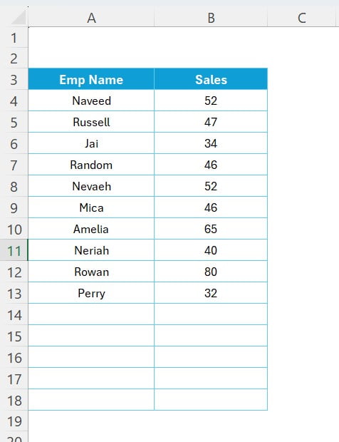
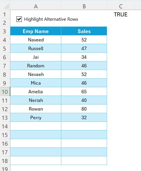
Let’s say we have some data points on range A3 to B18. Now, we want to highlight the alternative rows in this data using a check box. When we check the check box alternative rows should be highlighted. And, when we uncheck the check box then highlighted should be disappeared. Now, let’s start, how we can achieve this in Microsoft Excel.
Step -1: Inserting a Form Control Checkbox
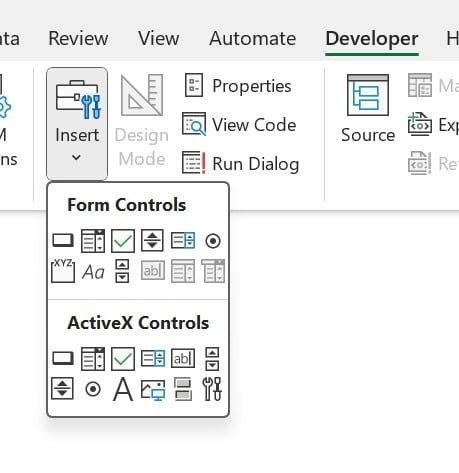
The adventure begins in the Developer tab within Excel. If you’ve not already enabled it, you can do so by right-clicking on the ribbon and selecting ‘Customize the Ribbon‘ to check the Developer option. Within the Developer tab, you’ll find the option to insert a form control checkbox. Drag this checkbox onto your Excel sheet and give it a purposeful name, such as “Highlight Alternative Rows.” This name serves as a clear instruction for the user, making your Excel sheet not only functional but also user-friendly.
Watch the below given video tutorial to learn how to enable the Developer tab in Excel:
Step -2: Link the Checkbox for Dynamic Interaction
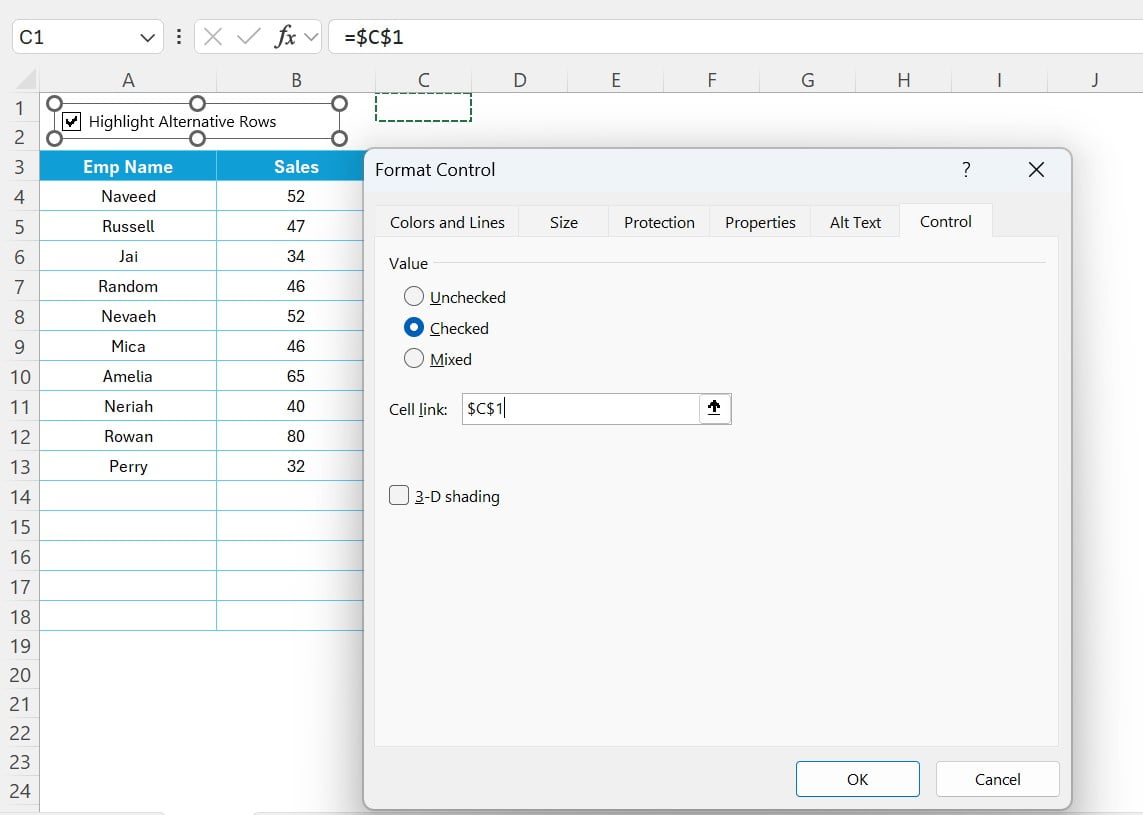
Once we have inserted the checkbox, the next step involves a bit of customization. So right click on the check box and click on format control. Now click on cell link box and linked with C1 range. Finelly, our checkbox is linked with the C1 cell. If you check this check box then you will see TRUE on C1 and if you uncheck this then there will be FALSE.
Step-3: Applying Conditional Formatting
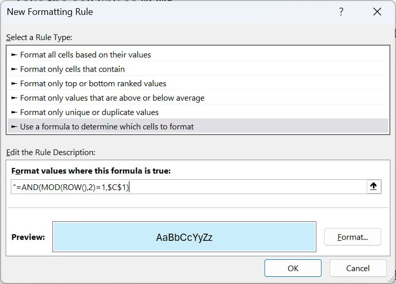
Now, with your checkbox configured, select the range A3:B18, the area of your data you wish to dynamically format. Press the shortcut keys Alt + O + D to open the Conditional Formatting Rules Manager. Here, you’ll create a new rule by selecting “Use a formula to determine which cells to format.” The magic formula “=AND(MOD(ROW(),2)=1,$C$1)” is what makes this entire process dynamic. It checks two conditions: whether the row is odd-numbered (for alternative row highlighting) and if the checkbox is checked (indicating user preference for highlighting).
Step 4: Format with Background color
Upon entering the formula, proceed to format these selected cells with a light blue background fill color (or any color of your preference) to visually distinguish the alternative rows. Once applied, this setting allows you to toggle the highlighting on and off, providing a dynamic and interactive way to view your data.
The Finale: Dynamic conditional formatting applied
Now, a dynamic conditional formatting is applied on your selected range. if you click on the check box then you will see alternative rows are highlighted with light blue color. As you uncheck the checkbox the light blue color will be disappeared.
Wrapping Up
This guide has walked you through the steps to dynamically highlight alternative rows in Excel using conditional formatting and a form control checkbox. By embracing these techniques, you’re not just working smarter with your data; you’re also unlocking new ways to present and analyze information effectively. Remember, the key to mastering Excel lies in exploring its vast array of features and creatively applying them to your data challenges. Happy Excel-ing!
By leveraging the power of Excel’s conditional formatting and the interactive capability of form control checkboxes, you can turn static data into dynamic visualizations. This guide aims not only to instruct but also to inspire you to explore further, making your data work for you in new and engaging ways.
Visit our YouTube channel to learn step-by-step video tutorials