Part of the free Module 11: Excel Dashboards · Lesson 5 of 10 · Full Excel course
Updated on 5 September 2026 · Works in Excel 365, 2021, 2019 and 2016 unless noted.
An incentive dashboard in Excel turns raw employee results into a payout using weighted scores, band tables and an eligibility rule. This Incentive Dashboard scores five metrics (calls, AHT, sales, quality score and client escalations), weights them, maps the total score to a percentage of the maximum payout, blocks employees with too many absences, and summarises total and average payout with a frequency chart and a speedometer. Every rule lives on one Weightage sheet so HR can change it without editing formulas.

How the incentive scheme works
Each metric carries a weightage and the weightages add up to 100 percent. An employee’s result on each metric is looked up in a band table and converted to a score out of that metric’s weightage. The five scores are summed into a Total Score, and the Total Score is looked up in a payout band table that returns a percentage of the maximum payout. Employees with three or more absences in the month are marked not eligible and receive nothing regardless of score.
| Metric | Direction | Sample weightage | Band example |
|---|---|---|---|
| Calls | Higher is better | 20% | 0 to 99 = 0, 100 to 149 = 10, 150+ = 20 |
| AHT | Lower is better | 20% | 0 to 300 = 20, 301 to 360 = 10, 361+ = 0 |
| Sales | Higher is better | 30% | 0 to 9 = 0, 10 to 19 = 15, 20+ = 30 |
| Quality | Higher is better | 20% | 0 to 79% = 0, 80 to 89% = 10, 90%+ = 20 |
| Client Escalation | Lower is better | 10% | 0 = 10, 1 = 5, 2+ = 0 |
The workbook structure
| Element | Technique | Formula or feature |
|---|---|---|
| Navigation | Shapes with hyperlinks on the Index sheet | Right-click shape, Link, Place in This Document |
| Metric score | Approximate-match lookup on a band table | =VLOOKUP(D2, Weightage!$A$10:$B$13, 2, TRUE) or XLOOKUP(D2, band_from, score, , -1) |
| Total Score | Sum of the five scores | =SUM(I2:M2) |
| Eligibility | Absence limit from Weightage | =IF(C2>=Weightage!$B$30, "Not Eligible", "Eligible") |
| Payout % | Approximate-match lookup on Total Score | =VLOOKUP(N2, Weightage!$A$34:$B$40, 2, TRUE) |
| Payout | Percent of max payout, zero if not eligible | =IF(O2="Eligible", P2*Weightage!$B$44, 0) |
| Summary cards | Shapes linked to Support cells | =SUM(Data!Q:Q), =AVERAGEIF(Data!O:O,"Eligible",Data!Q:Q) |
| Frequency chart | COUNTIFS per score band on the chosen metric | Combo box link + INDEX picks the metric column |
| Eligible % speedometer | Doughnut and pie overlay on Support cells | =COUNTIF(Data!O:O,"Eligible")/COUNTA(Data!A:A)-1 |
How each sheet is built
Index
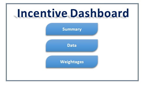
Three buttons, Summary, Data and Weightage, are shapes with hyperlinks to the respective sheets. The same shapes are copied to the top of every sheet so the reader can move around without the sheet tabs.

Summary
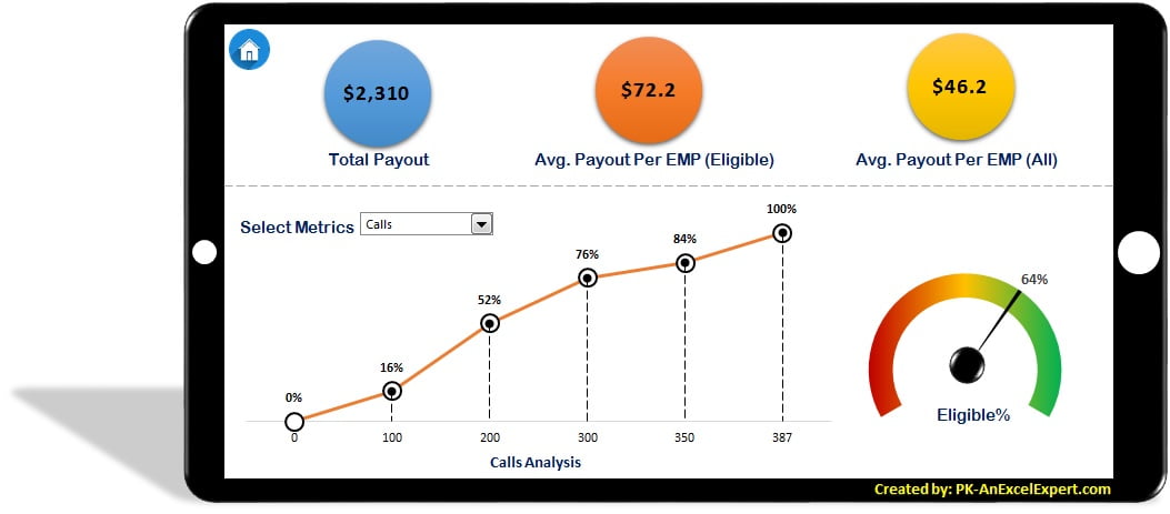
Three circular cards show Total Payout, Average Payout per Eligible Employee and the eligible count. A metric drop-down (Form Control combo box) drives a line chart of score frequency, showing how many employees fell into each score band for the chosen metric, and a speedometer chart shows the eligible employee percentage.

Data
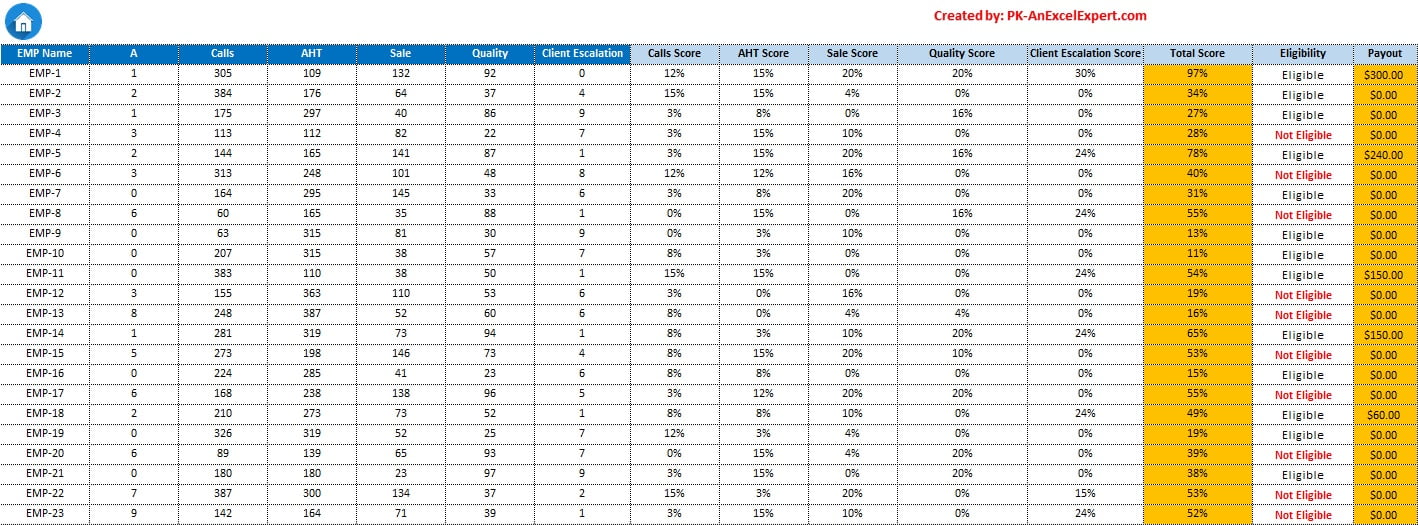
This is the calculation engine. The dark-blue Input columns are typed in: EMP Name, absences, Calls, AHT, Sale, Quality and Client Escalation. The sky-blue Formula columns compute each metric score with an approximate-match lookup against the band tables, then Total Score, Eligibility, Payout % and Payout. Colour-coding input and formula columns is a convention worth copying in every calculator you build.

Weightage
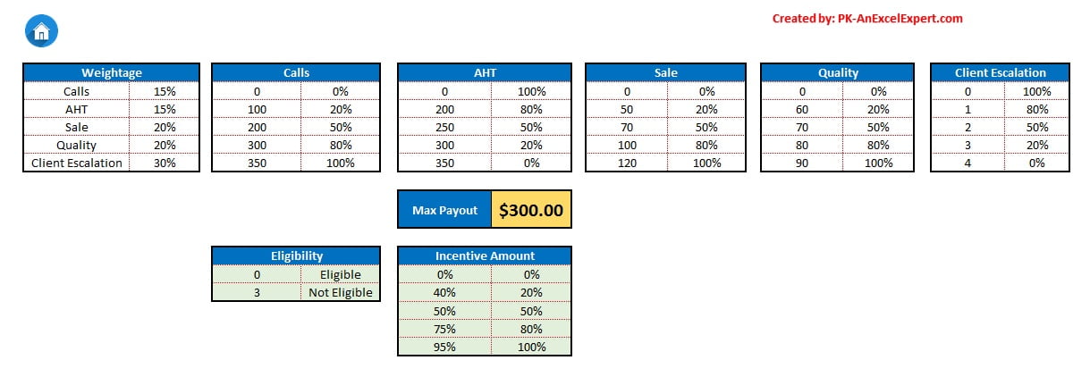
Nine small tables define the scheme:
- Weightage: the share of each metric; must total 100 percent.
- Calls, AHT, Sales, Quality and Client Escalation: banded lookup tables that turn a raw result into a score. The first column is the band start, sorted ascending.
- Eligibility: the absence limit; three or more absences means no payout.
- Payout amount %: Total Score bands against percent of maximum payout, for example 40 to 49 earns 20 percent.
- Max Payout: the ceiling amount per employee.

Support (hidden)
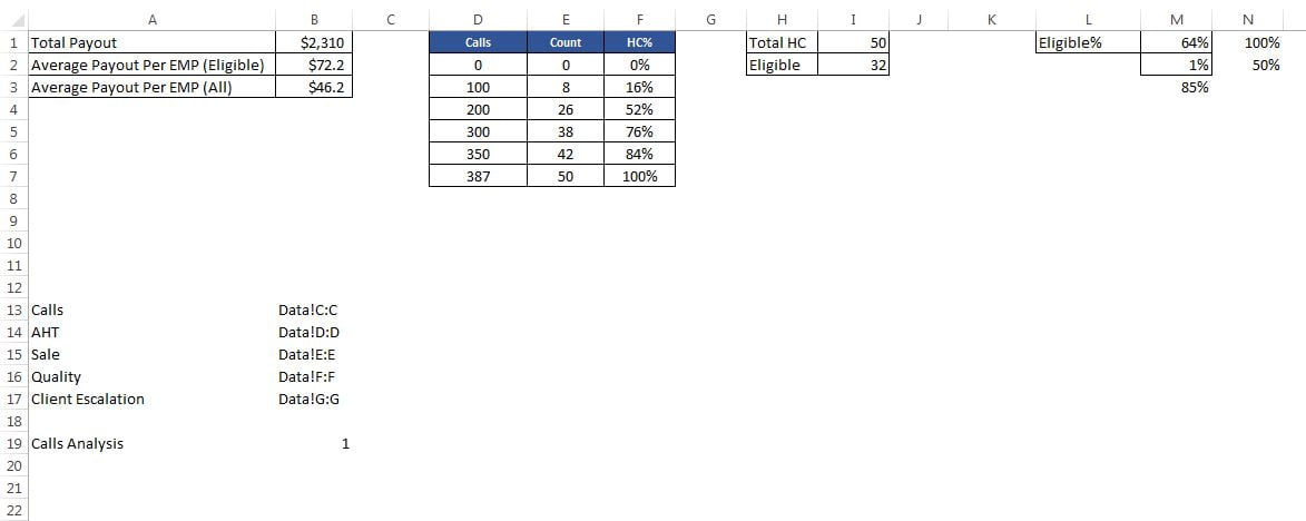
Helper calculations for the Summary cards, the frequency distribution (COUNTIFS per band for the metric picked in the combo box) and the three-cell series behind the speedometer.

Worked example
Using the sample weightages and bands in the table above, with a maximum payout of 5,000 and payout bands 0 to 39 = 0%, 40 to 59 = 20%, 60 to 79 = 50%, 80 to 100 = 100%:
| Employee | Absences | Calls | AHT | Sales | Quality | Escalations | Scores | Total | Payout |
|---|---|---|---|---|---|---|---|---|---|
| Asha | 1 | 160 | 290 | 22 | 92% | 0 | 20+20+30+20+10 | 100 | 5,000 |
| Ravi | 0 | 120 | 340 | 14 | 85% | 1 | 10+10+15+10+5 | 50 | 1,000 |
| Neha | 3 | 170 | 280 | 25 | 95% | 0 | 20+20+30+20+10 | 100 | 0 (not eligible) |
Ravi’s Total Score of 50 falls in the 40 to 59 band, so VLOOKUP(50, payout_table, 2, TRUE) returns 20 percent and the payout is 0.2 x 5,000 = 1,000. Neha scores full marks but has three absences, so the eligibility formula returns Not Eligible and the payout is zero. The Summary cards show Total Payout 6,000, Average Payout per Eligible Employee 3,000 and 2 of 3 eligible (66.7 percent on the speedometer).
How to use it with your own data
- On the Weightage sheet set your metric weightages (check they total 100 percent), the score bands, the absence limit, the payout bands and the maximum payout.
- On the Data sheet paste employee names and the month’s raw results into the dark-blue columns only.
- Fill the formula columns down if you added rows.
- Open Summary, choose a metric in the drop-down and review the payout totals and eligibility percentage.
- Copy the Payout column (Paste Values) to your payroll file.
Get the finished file
The finished Incentive Dashboard workbook is available as a ready-to-use template: Get the Incentive Dashboard in Excel. The five videos below show the complete build.
Watch the video
Tips and common mistakes
- Use approximate-match lookups (VLOOKUP with TRUE, or XLOOKUP with match mode -1) on the band tables, and keep the band starts sorted ascending.
- Lower-is-better metrics need reversed bands. AHT and escalations must award the highest score to the lowest values.
- Add a weightage check cell.
=IF(SUM(B3:B7)=1,"OK","Weightages do not total 100%")next to the table. - Protect the formula columns and the Weightage sheet (Review > Protect Sheet) so operators cannot overwrite the rules.
- Round at the end. Round the final payout to whole currency units, not each score step.
- Keep one month per file or add a Month column and filter; do not overwrite last month’s inputs without a copy.
Errors and how to fix them
| Symptom | Cause | Fix |
|---|---|---|
| Score shows #N/A | Result is below the first band start | Start every band table at 0 |
| Everyone gets the top score on AHT | Band table sorted for higher-is-better | Reverse the score column for lower-is-better metrics |
| Payout exceeds the maximum | Weightages total more than 100 percent | Fix the weightages; add the check cell |
| Eligible employee shows zero payout | Total Score below the first payout band | Check the payout band table starts at 0 with 0 percent |
| Frequency chart empty | Combo box link cleared | Pick a metric in the drop-down |
Practice exercise
- Add a sixth metric, Attendance %, with a 10 percent weightage, and rebalance the others so the total stays 100 percent.
- Replace the VLOOKUP score formulas with XLOOKUP (Excel 365 and 2021) using match mode -1.
- Add a Team column on Data and a SUMIFS block on Support that shows total payout per team.
- Add a conditional formatting icon set to the Total Score column so 80 and above shows a green tick.
Key takeaways
- Keep every rule (weights, bands, limits, ceilings) in tables on one sheet; formulas only look them up.
- Approximate-match lookups on a sorted band table are the cleanest way to convert a result into a score.
- Eligibility is a separate gate applied after scoring, so a top scorer can still receive zero.
- Colour-coded input and formula columns tell operators exactly where to type.
- The Summary sheet is only aggregation: SUM, AVERAGEIF, COUNTIF and two charts.
Related lessons
- Excel Dashboards course hub
- Performance Dashboard in Excel
- C-SAT Dashboard in Excel
- Excel dashboard checklist: test, protect and publish
- VLOOKUP function and AVERAGEIF function
- Speedometer chart in Excel
- Microsoft Support: VLOOKUP function
Frequently asked questions
How do I calculate incentive in Excel with weighted metrics?
Give each metric a weightage that sums to 100 percent, build a band table per metric that converts a result to a score out of that weightage, sum the scores, then look the total up in a payout band table to get a percentage of the maximum payout. This workbook does exactly that with VLOOKUP approximate matches.
Can I change the number of metrics?
Yes. Add a metric column and score column on Data, a band table and a weightage row on Weightage, include the new score in the Total Score SUM, and rebalance the weightages so they still total 100 percent.
What happens if the weightages do not total 100 percent?
Total Scores will be scaled up or down and the payout bands will not behave as intended. Add a check cell beside the Weightage table that flags when the sum is not 100 percent and colour it red with conditional formatting.
Is any VBA used?
No. Navigation uses hyperlinked shapes and all logic is formulas, so the file works in Excel 2010 through Microsoft 365 on Windows and Mac without enabling macros.
Should I use VLOOKUP or XLOOKUP for the band tables?
Both work. VLOOKUP with TRUE runs in every Excel version and needs the band starts sorted ascending. XLOOKUP with match mode -1 (exact or next smaller) does the same in Excel 365 and 2021 and does not need sorting, but the file will show #NAME? in older versions.
Want the finished version? Ready-made Excel dashboards, trackers and VBA systems are available at NextGenTemplates.com.