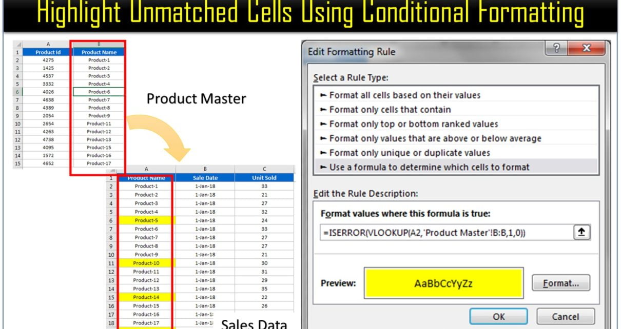
In this article you will learn how to Highlight Unmatched Cells Cells values from another range using Conditional formatting.
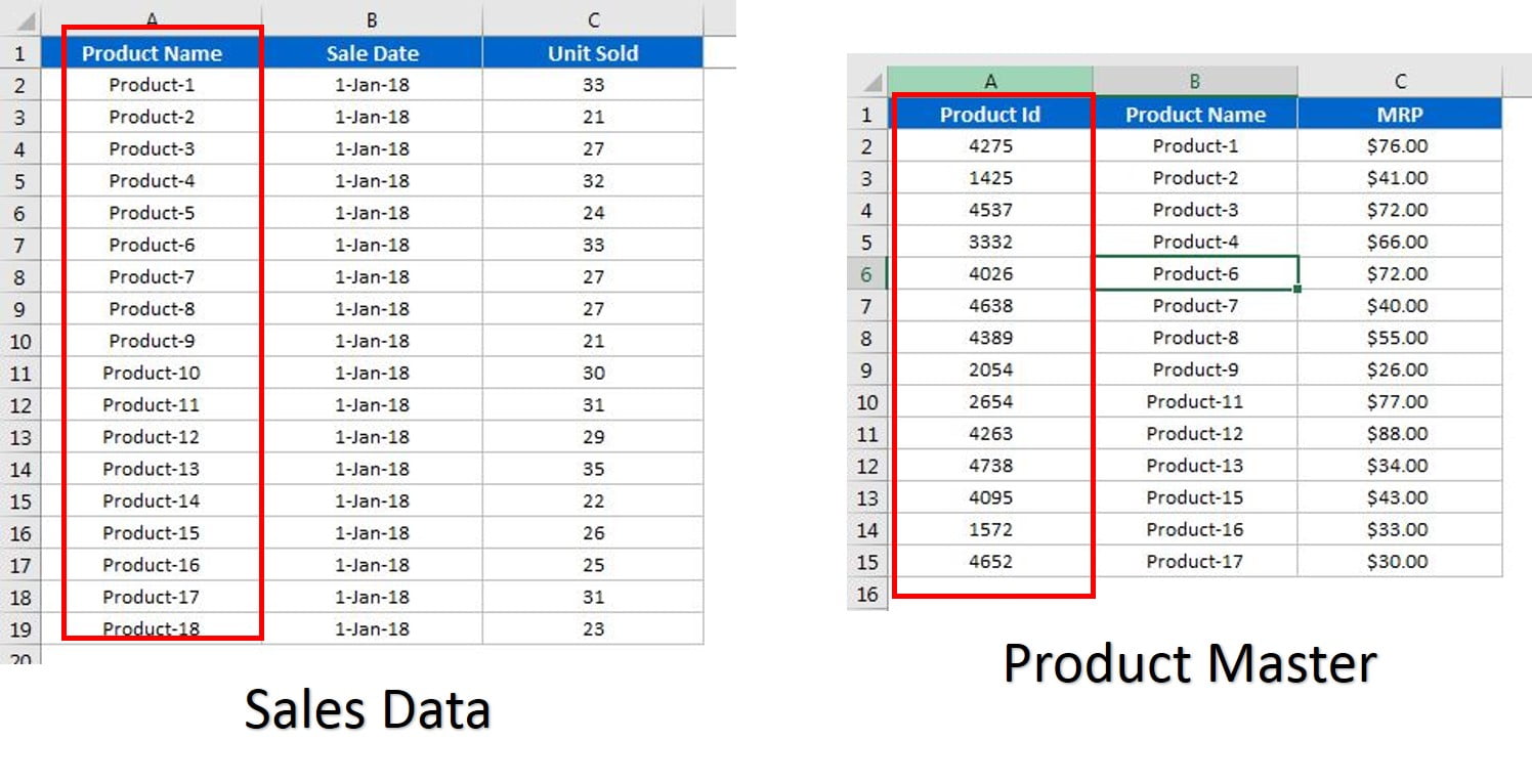
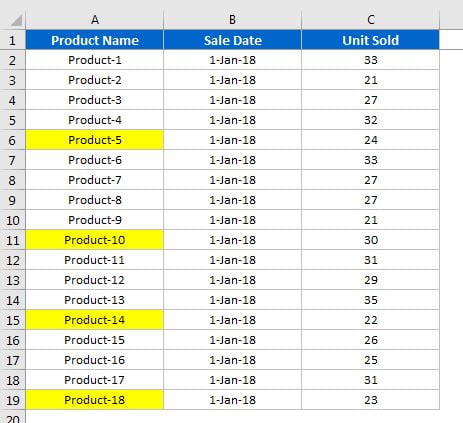
For Example, we have Sales and Product Master worksheets. In the Sales worksheet we need to highlight the Products which are not available in Product Master.
Highlight Unmatched Cells
Below are the steps to put the Conditional Formatting to highlight Product Name in Sales data-
- Select the Range (“A2:A19”)
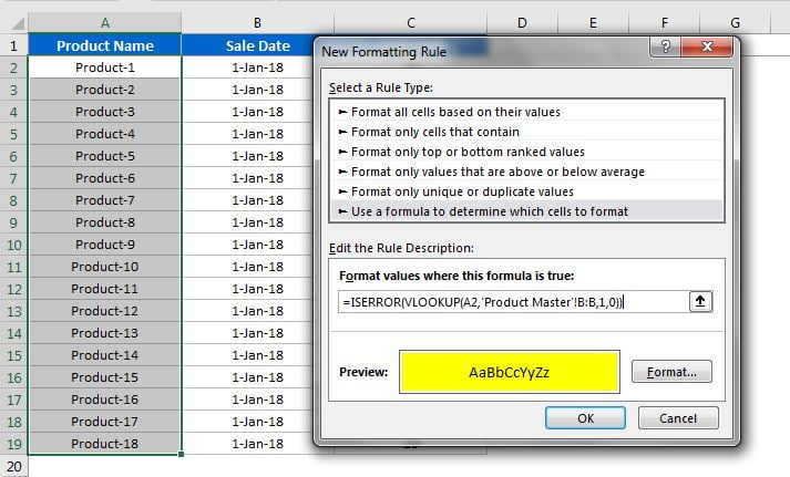
- Go to Home >> Conditional Formatting >> New Rule or Press Alt+D+O+N
- Select “Use a formula to determine which cells to format”
- Put any one of below given formula in the box.
- “=ISERROR(VLOOKUP(A2,’Product Master’!B:B,1,0))”
Or
- “=ISERROR(MATCH(A2,’Product Master’!B:B,0))”
Or
- “=COUNTIF(‘Product Master’!$B$2:$B$15,A2)=0”
- Click on Format button and select some background color.
- Click on OK.
Now Product Name which are not available in Product Master will be highlighted in Sales worksheet.
Click here to download the practice workbook.
Visit our YouTube channel to learn step-by-step video tutorials