Highlight Consecutive Duplicates in Excel with a Simple Formula

To highlight consecutive duplicates in Excel, you only need one conditional formatting rule with a short OR formula. It colours a value only when the same value sits directly above or below it, so a repeated month next to itself lights up, but the same month further down the list does not. In this tutorial you build that rule on a month-wise sales list, then use the same idea in an attendance sheet to highlight employees who take consecutive weekly offs (WO). Everything below follows PK’s video and the free practice workbook.

⬇️  Download the Practice Workbook
Excel workbook (.xlsx, 12 KB) · 2 sheets: month-wise sales and employee attendance · no macros

Watch the Video Tutorial

In the video PK tests the formula in a helper column first, turns it into a conditional formatting rule for the month list, and then adapts it to highlight only consecutive weekly offs in an attendance sheet.

What You Will Build

• A vertical rule that highlights a month when the same month is in the cell directly above or below it.
• A quick TRUE/FALSE test in a helper column, so you can see exactly what the rule will colour before you apply it.
• A horizontal rule for an attendance sheet that compares each day with the day before and the day after.
• A filtered rule that highlights only consecutive WO (weekly off) codes and ignores repeated P, A and L codes.

How the Practice File Is Laid Out

• Sheet1: Month in A1 and Sales in B1, with 29 rows of data in A2:B30. Months repeat in random order, for example Oct, Oct, Feb, Feb, Sep, Sep at the top.
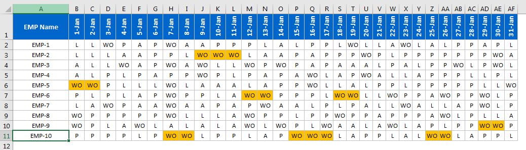
• Sheet2: EMP Name in A1, the dates 1-Jan to 31-Jan in B1:AF1, and ten employees (EMP-1 to EMP-10) in A2:A11. Each day holds an attendance code: P (present), A (absent), L (leave) or WO (weekly off).

Part 1: Highlight Consecutive Duplicates in Excel in a Column

The goal: if October appears in A2 and again in A3, both cells are highlighted because the second one comes right after the first. A Feb in row 8 and another Feb in row 13 are duplicates too, but they are not next to each other, so they stay white.

Step 1: Understand what the rule needs

A formula-based conditional formatting rule needs a logical formula, one that returns only TRUE or FALSE. Whenever the formula returns TRUE for a cell, Excel formats that cell. When it returns FALSE, the cell is left alone.

Step 2: Test the logic in a helper column

Before touching conditional formatting, PK checks the formula on the sheet. In C2 enter:

=OR(A2=A1,A2=A3)

Fill it down to C30. Rows 2 and 3 (Oct, Oct) return TRUE, rows 4 and 5 (Feb, Feb) return TRUE, and row 8 (a single Feb) returns FALSE. Type Feb into a cell next to another Feb and the result flips to TRUE straight away. Once you are happy with the results, copy the formula text and delete the helper column.

Step 3: Create the conditional formatting rule

1. Select A2:A30, starting the selection from A2 so that A2 is the active cell.
2. Go to Home > Conditional Formatting > New Rule. PK also uses the shortcut Alt+O+D, which opens the Conditional Formatting Rules Manager, where you click New Rule.
3. Choose Use a formula to determine which cells to format.
4. In Format values where this formula is true, paste =OR(A2=A1,A2=A3).
5. Click Format, open the Fill tab and pick a background colour (PK uses orange).
6. Click OK, then OK (or Apply in the Rules Manager).

How the formula works

• A2=A1 asks: is this month the same as the one directly above? This catches the second cell of a pair.
• A2=A3 asks: is this month the same as the one directly below? This catches the first cell of a pair.
• OR(...) returns TRUE if either test is TRUE, so both cells of a pair get coloured.
• The references are relative (no $ signs). Excel writes the rule for the active cell A2 and shifts it for every other cell, so A15 is checked with =OR(A15=A14,A15=A16). That is why the active cell must be A2 when you type the formula.

In the sample file the rule highlights Oct (rows 2-3), Feb (4-5), Sep (6-7), Sep (15-16), Jul (19-20) and Mar (25-27). Three equal months in a row are all highlighted, because the middle one matches both neighbours. Row 27 is typed as lowercase mar and is still highlighted: the = comparison in Excel is not case-sensitive.

A second example: random fruit names

PK also fills H3:H15 with random Apple, Banana and Mango values and highlights the consecutive duplicates there. The same logic works for any list of text or numbers. In the video he does this one with the Highlight Consecutive Duplicates button of his free PK’s Utility Tool add-in, which adds the same kind of rule in one click.

Part 2: Highlight Consecutive Weekly Offs in an Attendance Sheet

This is where the trick becomes really useful. When you build a roster or check attendance, you often need to see which employees have taken two or more weekly offs back to back. Here the data runs across the row (one column per day), so the formula compares left and right instead of up and down.

Step 4: Write the horizontal version

1. On Sheet2 select B2:AF11, with B2 as the active cell.
2. Open Home > Conditional Formatting > New Rule (or Alt+O+D > New Rule) and choose Use a formula to determine which cells to format.
3. Enter =OR(B2=A2,B2=C2), pick a fill colour and click OK.

The rule works, but it highlights every repeated code: two P days in a row, two A days, two L days. Most of the sheet turns orange, which is not what we want.

Step 5: Limit the rule to WO only

Open the Rules Manager again (Alt+O+D), select the rule, click Edit Rule and wrap the formula in AND with a second test:

=AND(OR(B2=A2,B2=C2),B2="WO")

Click OK. Now only weekly offs that sit next to another weekly off are highlighted.

How the formula works

• B2=A2 compares the day with the previous day (the column to the left). For 1-Jan the left cell is the employee name, which never equals WO, so the first day is handled safely.
• B2=C2 compares the day with the next day (the column to the right).
• OR(...) is TRUE when the code repeats on either side.
• B2="WO" is TRUE only when the code is a weekly off.
• AND(...) needs both tests to be TRUE, so a repeated P, A or L is ignored.

In the practice file this highlights EMP-2 on 9, 10 and 11 Jan, EMP-5 on 1 and 2 Jan, EMP-6 on 12-13 and 18-19 Jan, EMP-9 on 29-30 Jan, and EMP-10 on 7-8, 15-17 and 25-26 Jan. You can replace “WO” with any code you want to watch, such as “A” for consecutive absences.

Variations You Can Use (Addition)

These variations are additions to the video, based on standard Excel behaviour.

Highlight the whole row

Select A2:B30 and lock the column with a $ sign so every cell in the row checks column A: =OR($A2=$A1,$A2=$A3). The month and its sales value are both coloured.

Highlight only the repeat, not the first value

If you want the first Oct to stay white and only the repeat to be coloured, drop the second test: =A2=A1.

Make the match case-sensitive

Because = ignores case, Mar and mar count as the same. Use EXACT when case matters: =OR(EXACT(A2,A1),EXACT(A2,A3)).

Ignore blank cells

Two empty cells are equal, so blank rows inside the range get highlighted. Add a not-blank test: =AND(A2<>"",OR(A2=A1,A2=A3)).

Common Errors and Fixes

The wrong cells are highlighted, one row off

The active cell was not A2 when you typed the formula, so the relative references point to the wrong rows. Open Manage Rules, check that Applies to starts at A2 and that the formula refers to A2, then fix it.

Nothing is highlighted

Check for extra spaces or different spellings: “Sep” and “Sep ” (with a trailing space) are not equal. Use TRIM on the data, or test the formula in a helper column as in Step 2.

Every repeated code is highlighted in the attendance sheet

The rule is still the plain OR version. Edit it and add the WO test with AND, as in Step 5.

Tips

• Always test a conditional formatting formula in a spare column first. If the TRUE/FALSE results look right, the highlighting will be right.
• Use Alt+O+D (or Home > Conditional Formatting > Manage Rules) to see, edit and delete every rule on the sheet.
• Microsoft’s guide to using conditional formatting to highlight information covers every rule type and how to manage rules.

Want It Ready-Made?

If you track attendance every month, the free Weekly Attendance Sheet in Excel and the Employee Attendance Data Entry System in Excel on NextGenTemplates.com give you a ready structure to apply this rule to. Browse more HR and payroll templates in Excel. To get confident with logical formulas like OR, AND and EXACT, PK’s Excel AI Mastery: 100 Formulas course walks through them step by step.

Related Tutorials

• Highlight Duplicate or Unique Values in Excel
• Excel Conditional Formatting Formula: Highlight Rows
• Remove Duplicates in Excel and Highlight Duplicate Rows
• Attendance Tracker in Excel: Monthly Sheet Step by Step
• Highlight Unmatched Cells using Conditional Formatting

Frequently Asked Questions

What is a consecutive duplicate in Excel?

It is a value that is repeated in the very next cell, for example the same month in A2 and A3. A value that appears again later in the list, with other values in between, is a duplicate but not a consecutive one.

Which formula highlights consecutive duplicates in a column?

Use OR to compare each cell with the cell above and the cell below, for example =OR(A2=A1,A2=A3) for a list that starts in A2. Apply it with Use a formula to determine which cells to format, as shown in Step 3.

How do I highlight consecutive duplicates in a row instead of a column?

Compare each cell with the cells to its left and right instead, for example =OR(B2=A2,B2=C2) for a range that starts in B2. Part 2 of this tutorial uses exactly this for an attendance sheet.

How do I highlight only consecutive weekly offs and not other codes?

Wrap the OR test in AND and add a second test that checks the cell equals the weekly off code. Step 5 shows the full formula for the WO code.

Does the rule highlight three or more equal values in a row?

Yes. Every cell in a run has at least one equal neighbour, so the whole run is coloured, as with the three March entries in the practice file.

About the Author

PK is a Microsoft Excel expert and trainer and the founder of PK: An Excel Expert and NextGenTemplates.com. He has been teaching Excel, VBA, Power Query and Power BI since 2016 on his YouTube channel. For more rules like this one, see his free conditional formatting course.

Conclusion

To highlight consecutive duplicates in Excel, select the range with the first data cell active and add a formula rule that compares each cell with its neighbours: =OR(A2=A1,A2=A3) for a column, =OR(B2=A2,B2=C2) for a row. Wrap it in AND with a code test, like B2=”WO”, and the same rule shows you exactly which employees take back-to-back weekly offs. Download the practice workbook, try both sheets, and adapt the rule to your own rosters and lists.