Attendance Tracker in Excel: Monthly Sheet with Data Bars

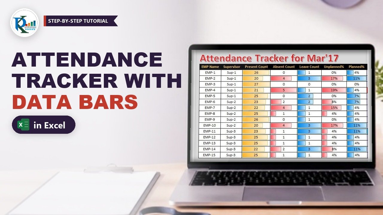
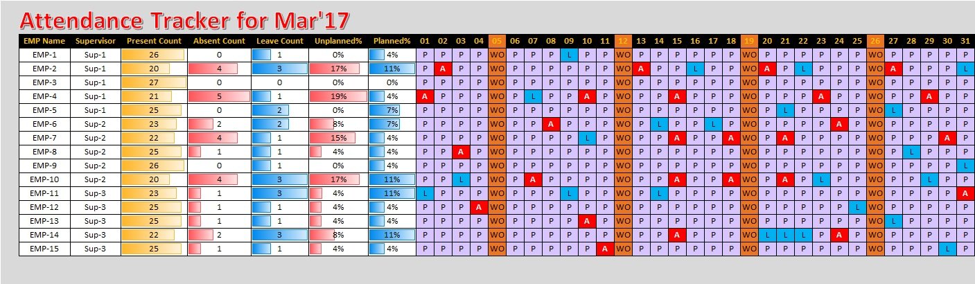
An attendance tracker in Excel gives you one sheet where you mark every employee’s day and instantly see who was present, who was absent and how much leave was taken. In this tutorial you build PK’s monthly tracker from a blank sheet: a 31-day date grid, a P/A/L/WO drop-down, Sundays highlighted automatically, colour-coded attendance codes, COUNTIF totals, Unplanned% and Planned% formulas, and data bars that make the summary easy to scan. Everything uses built-in features, with no VBA.

Watch the Video Tutorial

In the video PK sets up the headers and dates, adds the drop-down and the Sunday rule, colours the codes, writes the COUNTIF and percentage formulas, adds data bars and finishes the design.

What You Will Build

• A monthly grid with one row per employee and one column per day.
• A drop-down list so every cell holds a valid code: P, A, L or WO.
• Automatic Sunday highlighting driven by the date in the header.
• Present, Absent and Leave counts with COUNTIF.
• Unplanned% and Planned% per employee, with data bars for a quick visual read.

How the Attendance Tracker in Excel Is Laid Out

While you build, keep everything in row 1 and the columns below (the final design inserts a spacer column and two title rows later):

• A EMP Name and B Supervisor, typed by hand.
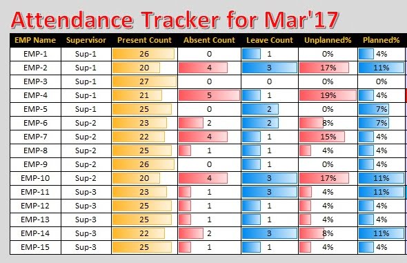
• C Present Count, D Absent Count, E Leave Count, F Unplanned % and G Planned %, all formulas.
• H1:AL1 the 31 dates of the month, and H2:AL16 the daily attendance for 15 employees.

Part 1 – Headers and Dates

Step 1: Type the headers and names

In A1:G1 type EMP Name, Supervisor, Present Count, Absent Count, Leave Count, Unplanned % and Planned %, and turn on Wrap Text so the headers stay narrow. Type EMP-1 in A2 and drag it down to EMP-15. In column B the sample uses three supervisors, Sup-1 to Sup-3, with five employees each.

Step 2: Create the date row

Type the first day of the month in H1 (the sample uses 3/1/2017, which is 1 March 2017) and fill the next cells with a simple formula:

H1  3/1/2017
I1  =H1+1

Copy I1 across to AL1 for 31 days. Then select H1:AL1, press Ctrl+1 (PK uses the older shortcut Alt+O+E), choose Custom and type dd. Each header shows only 01, 02, 03 and so on, but it is still a real date, which the Sunday rule in Part 2 depends on.

Part 2 – Drop-Down and Sunday Highlight

Step 3: Add the attendance drop-down

Select H2:AL16 and go to Data > Data Validation. Under Allow choose List and in Source type the four codes separated by commas:

P,A,L,WO

P is present, A is absent, L is leave and WO is the weekly off. Now each cell offers a drop-down, and anything else is rejected, which keeps the counts accurate.

Step 4: Highlight every Sunday

Select the date area including the header (H1:AL16), go to Home > Conditional Formatting > New Rule > Use a formula to determine which cells to format and enter:

=TEXT(H$1,"ddd")="Sun"

Choose an orange fill. Every Sunday column lights up from top to bottom.

How the formula works

• TEXT(H$1,"ddd") turns the date in the header into a three-letter day name such as Wed or Sun.
• The dollar sign before the row number locks the rule to row 1, while the column stays relative. So every cell in a column looks at its own date in the header.
• When the day name is Sun, the rule is TRUE and the whole column gets the fill. Change the month in H1 and the highlighted columns move by themselves.

Part 3 – Colour the Attendance Codes

With H2:AL16 still selected, add three rules with Conditional Formatting > New Rule > Format only cells that contain, Cell Value equal to:

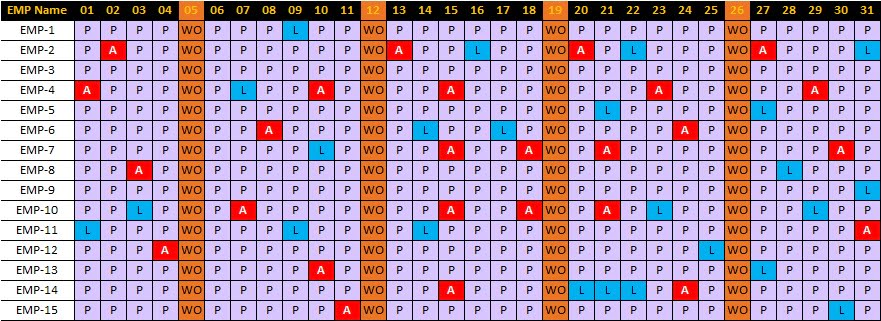
• P – a light violet fill.
• L – a blue fill.
• A – a red fill with a white font, so absences stand out the most.

Mark the Sundays as WO and fill in the rest of the month. The grid now reads like a heat map: a row with several red cells is easy to spot.

Part 4 – Attendance Tracker Formulas

Step 5: Count present, absent and leave days

Enter these in row 2 and copy them down to row 16:

C2  =COUNTIF(H2:AL2,"P")
D2  =COUNTIF(H2:AL2,"A")
E2  =COUNTIF(H2:AL2,"L")

COUNTIF counts how many cells in the employee’s row match the code. Because the drop-down allows only valid codes, these totals are always reliable.

Step 6: Calculate Unplanned% and Planned%

F2  =D2/(C2+D2)
G2  =E2/(C2+D2+E2)

Format both columns as percentages and copy them down.

How the formula works

• Unplanned% divides the absent days by the scheduled days, which are the present days plus the absent days.
• Planned% divides the leave days by present plus absent plus leave, which is everyone except the weekly offs. Week-offs are left out of both formulas because nobody was expected to work.
• Example from the video: EMP-1 has 13 present, 11 absent and 3 leave days, so Unplanned% is 11 / 24 = 46% and Planned% is 3 / 27 = 11%.

Step 7: Freeze the headers

Click H2 and choose View > Freeze Panes > Freeze Panes. The names, the summary columns and the date row stay in view while you scroll through the month.

Part 5 – Data Bars and Final Design

Step 8: Add data bars

Select each summary column and go to Home > Conditional Formatting > Data Bars. PK uses an orange bar for Present Count, red for Absent Count and Unplanned%, and blue for Leave Count and Planned%, so the colours match the daily grid.

Step 9: Polish the layout

• Turn off Gridlines and Headings in the View tab and hide the unused rows and columns.
• Insert two rows above the table and a narrow column A (width 3) for spacing, and give the surrounding area a grey fill.
• Colour the header row, add a WordArt title such as Attendance Tracker for Mar’17 and set the row height to 25.

Common Errors and Fixes

Sundays are not highlighted

The header holds text, not a date, or the rule lost its dollar sign. Make sure H1 is a real date and the rule reads H$1 with the dollar before the row only.

#DIV/0! in Unplanned% or Planned%

An employee has no P, A or L marked yet, so the denominator is zero. Wrap the formula in IFERROR, for example =IFERROR(D2/(C2+D2),0) (an addition, not in the video).

The counts look too low

A code was typed with a space or pasted from another file, which bypasses the drop-down. Use Data > Data Validation > Circle Invalid Data to find those cells.

Tips

• To reuse the sheet for another month, change only H1; the dates and Sunday columns follow.
• For months shorter than 31 days, clear or hide the extra date columns so they do not get marked by mistake.
• If your weekly off is Friday or Saturday, change Sun in the rule to Fri or Sat.
• Read Microsoft’s guide to applying data validation to cells for more drop-down options.

Want It Ready-Made?

If you would rather start with the finished file, the Attendance Tracker in Excel template on NextGenTemplates.com is ready to use. For a form-based system with entry screens and reports there is the Employee Attendance Data Entry System in Excel, or browse all HR and payroll Excel templates. To master COUNTIF, TEXT, IFERROR and other everyday formulas step by step, join the video course Excel + AI Mastery: 100 Essential Formulas and Real-World Projects.

Related Tutorials

• Attendance Sheet in Excel: 7 Methods Compared
• Weekly Attendance Sheet in Excel (Auto-Calculating)
• Absenteeism Report in Excel with Pivot Tables
• Highlight Dates in Excel: Due Today, Overdue, This Week and Weekends
• Excel COUNTIF Function with Examples

Frequently Asked Questions

How do I make an attendance tracker in Excel?

Put employee names in rows and the dates of the month in columns, add a drop-down with codes such as P, A, L and WO, then count each code per row with COUNTIF. Conditional formatting colours the codes and highlights the weekly off.

How do I highlight Sundays automatically?

Select the date area and add a conditional formatting rule that turns the header date into a day name with the TEXT function and the ddd format, then tests whether it equals Sun. Step 4 shows the exact formula. The rule checks the date in the header of each column.

How is the unplanned absence percentage calculated?

Absent days divided by present plus absent days. Leave and weekly offs are not part of the scheduled days, so they are left out of this formula.

Why are weekly offs excluded from Planned%?

Nobody is expected to work on a weekly off, so counting it would understate the leave rate. Planned% divides leave by present plus absent plus leave days only.

Can I use this tracker for any month?

Yes. Change the first date in H1 and the date headers and Sunday columns update. For shorter months, clear or hide the extra date columns.

About the Author

PK is a Microsoft Excel expert and trainer and the founder of PK: An Excel Expert and NextGenTemplates.com. He has been teaching Excel, Power Query and Power BI since 2016 on his YouTube channel.

Conclusion

An attendance tracker in Excel needs only a few building blocks: a date row, a drop-down for the codes, conditional formatting for Sundays and colours, COUNTIF for the totals and two simple percentage formulas. Add data bars and a clean layout, and you have a monthly sheet your whole team can read at a glance.