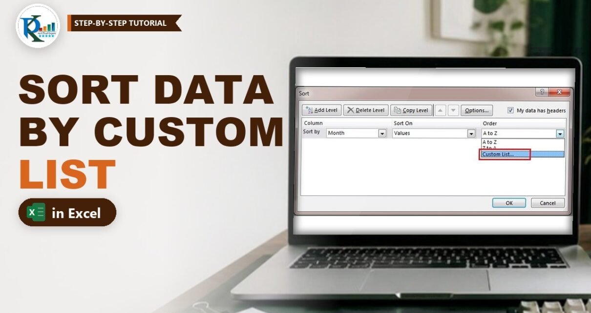
When you sort data by custom list in Excel, you choose the order yourself instead of accepting A to Z. That matters for month names, T-shirt sizes, priority levels and any other text that has a natural order. Month names typed as Jan, Feb, Mar are text, so a normal ascending sort gives you Apr, Aug, Dec, and a descending sort gives you Sep, Oct, Nov. No helper column is needed to fix this. In this tutorial you sort a monthly report Jan to Dec with Excel’s built-in month list, then create your own custom list (S, M, L, XL, XXL, XXXL) and sort a sizes table with it.
⬇️ Download the Practice Workbook
Two sheets (months and sizes) · .xlsx (no macros) · Excel 2010 and later
Watch the Video Tutorial
The video shows how to create your own custom list in Excel Options, by typing the entries or importing them from a range, and how the fill handle then repeats that list for you.
What You Will Learn
- Why a normal A to Z sort puts month names in the wrong order.
- How to sort a table by month with the built-in Jan, Feb, Mar custom list.
- How to create your own custom list, such as clothing sizes, in Excel Options.
- How to sort any column by that list, and how the same list fills cells with the fill handle.
- A formula alternative with SORTBY and MATCH for Microsoft 365.
The Practice Data
The workbook has two sheets:
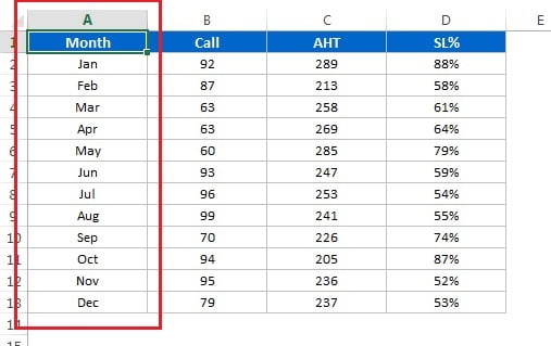
- Sheet1: a monthly call-centre report in A1:D13 with the headers Month, Call, AHT and SL%. The months are short names (Jan to Dec).
- Sheet2: a sizes table in A1:B25 with the headers Size and Unit, four rows each for S, M, L, XL, XXL and XXXL.
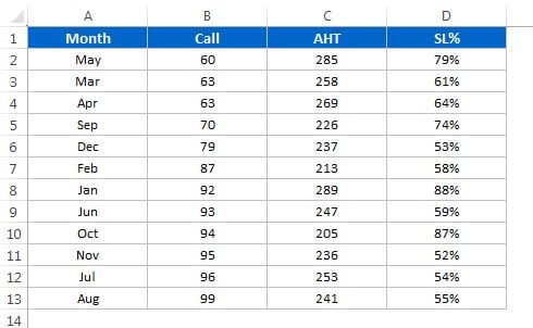
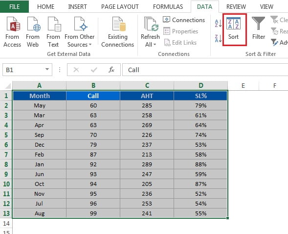
To practise, first shuffle a sheet, for example sort it by the numbers column. In the screenshot below the report is sorted by Call (smallest first), so the months are mixed up: May, Mar, Apr, Sep and so on.
Why A to Z Does Not Work for Months
Excel sorts text letter by letter. To Excel, Apr comes before Aug because p comes before u, and both come before Dec. So an ascending sort gives Apr, Aug, Dec, Feb, Jan, Jul, Jun, Mar, May, Nov, Oct, Sep, and a descending sort starts with Sep, Oct, Nov. Neither is calendar order.
A custom list fixes this. It is a saved sequence of values that tells Excel the order you want. Excel already ships with four of them: short day names, full day names, short month names and full month names.
Part 1: Sort Data by Custom List (Months)
Step 1: Select the data and open Sort
Click any cell in the table, or select the whole range A1:D13, then go to Data > Sort.
Step 2: Choose the column and Custom List
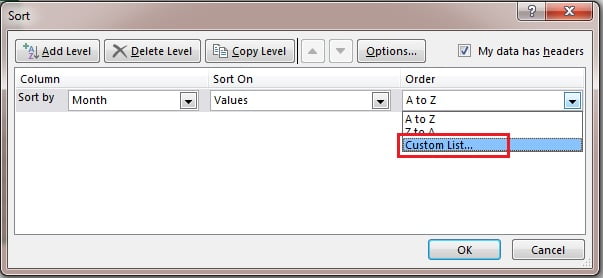
The Sort window opens. Make sure My data has headers is ticked, so row 1 stays on top. Then set:
- Sort by: Month
- Sort On: Values (Cell Values in newer versions)
- Order: Custom List…
Step 3: Pick the month list
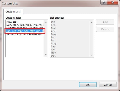
The Custom Lists window opens. Select Jan, Feb, Mar, Apr, May, Jun… because the data uses short month names. If your column had full names (January, February), you would pick the full-name list instead. Click OK.
Step 4: Confirm the sort
Back in the Sort window, the Order box now shows the month list. Click OK. The table is sorted Jan to Dec, and Call, AHT and SL% move with their months, as in the first screenshot of this post.
Part 2: Create Your Own Custom List
The built-in lists cover days and months only. For anything else, such as sizes, regions or a priority scale, you create the list once and Excel remembers it.
Step 5: Open Edit Custom Lists
Go to File > Options > Advanced. Scroll down to the General section and click Edit Custom Lists….
Step 6: Type or import the entries
With NEW LIST selected on the left, you have two ways to add a list:
- Type it in the List entries box, pressing Enter after each item. In the video PK types S, M, L, XL, XXL and XXXL, then clicks Add.
- Import it from cells: select a range in the Import list from cells box (the video uses
$D$4:$D$21, a list of Indian states) and click Import.
Click OK twice to close the windows. The four built-in lists are greyed out and cannot be edited, but the lists you add can be edited or deleted later from the same window.
Step 7: Fill a list with the fill handle
A custom list also works with AutoFill. Type any item, for example XL, and drag the fill handle down. Excel continues XXL, XXXL and then starts again at S, M, L. The same happens with Low, Medium, High or with a list of states.
Part 3: Sort the Sizes Table with Your List
Step 8: Sort by the new list
Go to Sheet2, shuffle it (sort by Unit, for example), then open Data > Sort again. Choose Sort by Size and Order Custom List…, select S, M, L, XL, XXL, XXXL and click OK twice. The rows now run S, M, L, XL, XXL, XXXL instead of the alphabetical L, M, S, XL, XXL, XXXL.
To sort the units inside each size as well, click Add Level, choose Then by Unit and order Smallest to Largest.
Modern Excel Alternative: SORTBY and MATCH
This formula is an addition, not part of the original file or video. In Microsoft 365 or Excel 2021 you can return a sorted copy without touching the original data. On Sheet1, enter this in F2:
=SORTBY(A2:D13,MATCH(A2:A13,{"Jan","Feb","Mar","Apr","May","Jun","Jul","Aug","Sep","Oct","Nov","Dec"},0))For the sizes on Sheet2:
=SORTBY(A2:B25,MATCH(A2:A25,{"S","M","L","XL","XXL","XXXL"},0))How the formula works
MATCH(A2:A13,{...},0)finds the position of each month in the array you typed: Jan returns 1, Feb returns 2, Dec returns 12. The 0 means exact match.SORTBYsorts the whole table A2:D13 by those positions, smallest first, so the rows come back in calendar order.- The result spills into F2:I13 and updates when the source data changes. Leave that block empty or you get a #SPILL! error.
You can also keep the order in a range, for example H2:H7, and use MATCH(A2:A25,H2:H7,0) so the order is easy to edit.
Common Errors and Fixes
Only one column was sorted
If you select just the Month column, Excel shows a Sort Warning. Choose Expand the selection, otherwise the months move and the numbers stay where they were.
Some rows end up at the bottom
Values that do not exactly match a list entry are placed after the listed ones. Look for extra spaces, a typo or a different spelling, such as Sept instead of Sep. TRIM removes stray spaces.
The header row moved into the data
My data has headers was not ticked. Undo with Ctrl + Z, tick the box and sort again.
My custom list is missing on another computer
Lists you create in Excel Options are saved in Excel on your own PC, not in the workbook. Add the list on the other computer, or use the SORTBY formula, which carries its order inside the formula.
Tips
- After choosing a custom list in the Sort window, open the Order drop-down again: Excel also offers the reverse order, for example Dec, Nov, Oct.
- Import long lists (products, branches, employees) from a range instead of typing them.
- Custom lists also control the order of items in pivot tables, so sizes and months appear in the right sequence there too.
- Delete a list you no longer need from the same Edit Custom Lists window.
- Microsoft explains the same feature in Sort data using a custom list.
Want It Ready-Made?
If you would rather start from finished, well-organised workbooks, browse the Excel templates on NextGenTemplates.com. To get confident with SORTBY, MATCH and the other dynamic array formulas used above, join the video course Excel + AI Mastery: 100 Essential Formulas and Real-World Projects.
Related Tutorials
- AutoFill in Excel: Fill Handle and Custom Lists
- Fill Series in Excel
- Quick Re-Arrange Columns Sequence Using Data Sorting
- MATCH Function in Excel with Examples
- VBA Sort and AutoFilter: Sort and Filter Data in Code
Frequently Asked Questions
How do I sort months in calendar order in Excel?
Select the table, go to Data, Sort, choose the month column, set Order to Custom List and pick the month list that matches your data (short or full names). Click OK twice and the rows run January to December.
Why does Excel sort months alphabetically?
Month names typed as text are just words to Excel, so it sorts them letter by letter. A custom list tells Excel the real order. Months stored as real dates sort correctly with a normal ascending sort.
How do I create a custom list in Excel?
Go to File, Options, Advanced, scroll to the General section and click Edit Custom Lists. Type the entries with Enter between them, or import them from a range, then click Add and OK.
Can I edit the built-in custom lists?
No. The four built-in day and month lists are locked. Lists you add yourself can be edited or deleted at any time.
Is the custom list saved in my workbook?
No. It is saved in Excel on your computer and is available in every workbook you open there. On another PC you need to add it again or use a formula such as SORTBY with MATCH.
About the Author
PK is a Microsoft Excel expert and trainer and the founder of PK: An Excel Expert and NextGenTemplates.com. He has been teaching Excel, VBA, Power Query and Power BI since 2016 on his YouTube channel.
Conclusion
To sort data by custom list in Excel, open Data > Sort, choose your column and set Order to Custom List. Use the built-in month and day lists, or create your own list once in File > Options > Advanced and reuse it for sorting and filling. Download the practice workbook, shuffle the months and sizes, and sort them back into the order that makes sense.