In this article, you will learn how to get the Quick date formats using formula in single cell. Excel is a powerful tool with the various function to get the required result. It is quite useful in the field of data analysis and reporting. When we work in a report, one common comes to manipulating date formats to fit various reporting needs. Have you ever found yourself needing to present dates in multiple formats within a single report? If so, you’re in luck! Our latest tutorial, “Quick date formats using formula in single cell,” simplifies this process, ensuring your reports are both comprehensive and efficient.
Also learn:
Dive into Date Formats Like Never Before
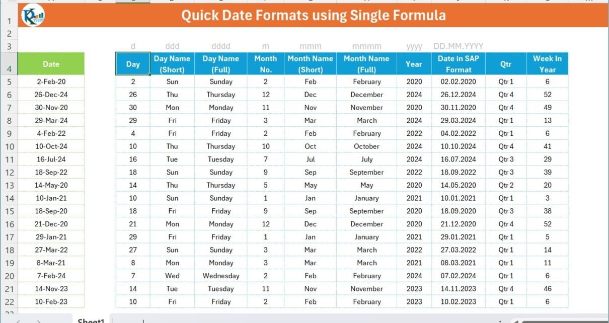
In this scenario, let’s say you have a range of dates in your Excel sheet, on A5 to A22. Now, You want to convert these dates into various formats, like day number, day name (both short and full), month number and name, year, and even the week number in the year. Moreover, you aim to include specialized formats like SAP date format also.
The Magic Formula Unveiled
To achieve this without manually converting each date, we introduce a game-changing formula that works wonders in a single cell. Imagine populating the range C5:L22 with all the date formats you need, using just one formula. Sounds like a dream, right? But it’s entirely possible, and we’ve done just that!
Here’s a sneak peek at what we’ve accomplished:
- Day, Day Name (Short and Full)
- Month No., Month Name (Short and Full)
- Year
- Date in SAP Format
- Quarter
- Week In Year
All these elements are neatly organized and presented in your Excel sheet, ready to elevate your data presentation game.
Date formats using formula in single cell
To achieve all the information in the single cell formula, we have used below given formula
=HSTACK(TEXT(Date,HSTACK(C3:J3)),"Qtr"&ROUNDUP(MONTH(Date)/3,0),MAP(Date,Week_In_Year))
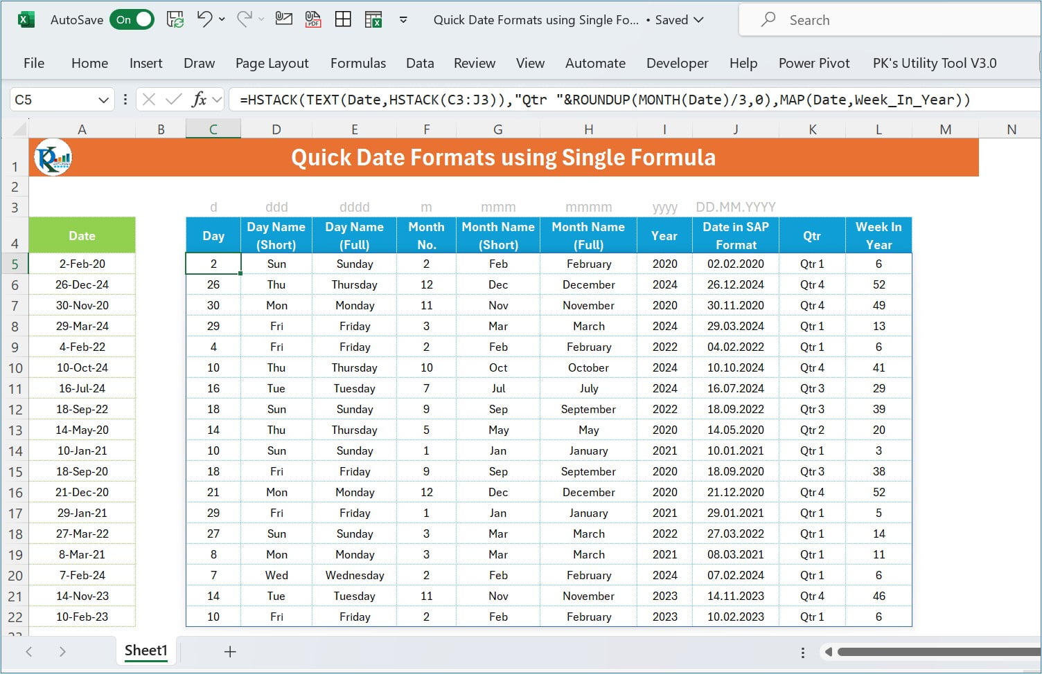
Now Let’s break it down in the 3 parts: Inside the first HSTACK formulas, we have used below given 3 formulas-
The TEXT and HSTACK Combo:
The first part of the formula is “TEXT(Date,HSTACK(C3:J3))”. TEXT function is used to format the number or date into a defined format. Here we have already taken the format on the range C3:J3. But in the Text function, we can put only single format at a time. So, to get the rid of this problem, we have used HSTACK function to use multiple criteria at a time.
Quarter Calculation:
The formula continues with “Qtr “&ROUNDUP(MONTH(Date)/3,0), a smart way to calculate the quarter of each date. It simply divides the month number by three and rounds up to the nearest whole number, giving you the quarter.
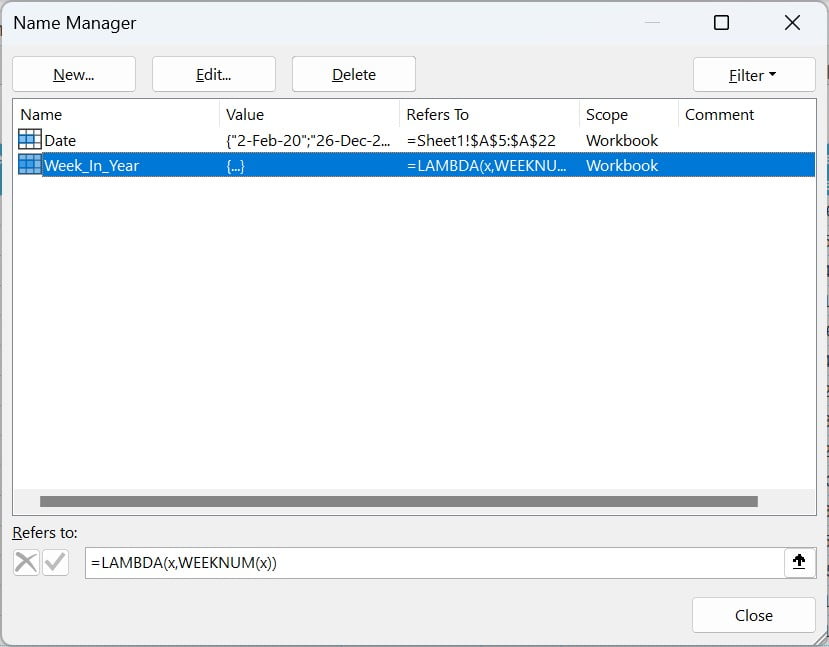
Week Number:
Finally, we calculate the week number in the year using MAP(Date,Week_In_Year). The MAP function iterates over each date, applying the custom LAMBDA function Week_In_Year, which we’ve predefined in Excel’s Name Manager to return the week number.
Why This Matters
It is quite useful technique, to combining the multiple formulas into one using the HSTACK function. In this article, we have explained the multiple things like getting the Month Name, Qtr or Week number. So, now in your report whenever you required anything like this you can use easily. This method not only streamlines your workflow but also enhances the readability and professionalism of your reports.
Engage and Excel
Now that we’ve shared this transformative approach with you. So, now it’s your turn to apply it in your daily work. You can apply it in your business dashboard or business report as per the requirements. As we know, Excel is a tool of endless possibilities, and mastering such techniques opens doors to advanced data manipulation and presentation skills. So, go ahead, give it a try, and take your Excel proficiency to new heights!
Conclusion
Remember, the world of Excel is vast and filled with opportunities to streamline and innovate. We always share the such tutorials in our website and on YouTube channel regularly. You can follow us to get the regular update of our videos and tutorials. Techniques like the one we’ve shared today are just the beginning. Stay curious, keep learning, and never underestimate the power of a well-formulated Excel cell. Happy Excel-ing!
Visit our YouTube channel to learn step-by-step video tutorials
Watch the step-by-step video tutorial:
Click here to download the practice file