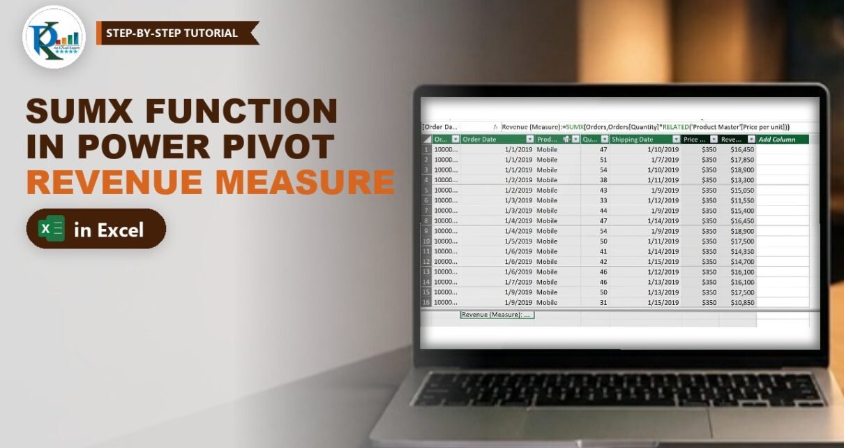
The SUMX function in Power Pivot lets you calculate revenue with a single measure, without adding any helper columns to your data. In this tutorial you load an Orders table and a Product Master table from two text files, link them with a relationship, and write one DAX measure that multiplies each order’s quantity by its product price and adds up the results. You then check the measure against the calculated-column method from the previous tutorial, and turn it into a PivotTable and a 3-D pie chart of revenue by product.
⬇️ Download the SUMX Practice Files
ZIP · SUMX FUNCTION.xlsx (Power Pivot data model, no macros) plus Orders.txt and Product Master.txt
Watch the Video Tutorial
PK imports both Notepad files into Power Pivot, creates the relationship, writes the SUMX measure, compares it with a calculated column and builds a pie chart from the measure.
What You Will Build
- A data model with Orders (the fact table) and Product Master (the lookup table), both imported from text files.
- A relationship between the two tables on Product.
- A Revenue measure using SUMX and RELATED: no price or revenue columns needed.
- A PivotTable that proves the measure matches the calculated-column result.
- A 3-D pie chart of revenue by product with percentage labels.
The Sample Data
The ZIP contains two tab-separated text files and the finished workbook:
- Orders.txt – 972 orders with Order Id, Order Date, Product, Quantity and Shipping Date.
- Product Master.txt – one row per product: Tablet 300, Mobile 350 and Laptop 600 per unit.
Revenue is Quantity × Price per unit, but quantity and price live in different tables. That is exactly the situation SUMX with RELATED handles.
Understanding the SUMX Function
SUMX returns the sum of an expression evaluated for each row of a table. The syntax is:
SUMX(<table>, <expression>)- table – the table whose rows SUMX loops through. It can be a table name or any expression that returns a table, such as a FILTER.
- expression – the calculation done for each row. It is not just a column: it can be any expression that returns a number, like quantity multiplied by price.
SUMX is an iterator. It visits each row of the table, calculates the expression for that row, and then adds all the row results together. Plain SUM can only add up one existing column; SUMX can add up a calculation.
Part 1 – Load the Text Files into Power Pivot
Step 1: Open the Power Pivot window
Start a new workbook and go to Power Pivot → Manage (Manage Data Model).
Step 2: Import Orders.txt
- Click Home → Get External Data → From Other Sources.
- In the Table Import Wizard scroll to the bottom, select Text File and click Next.
- Click Browse and pick Orders.txt.
- Tick Use first row as column headers and set the Column Separator to Tab. Check the preview.
- Click Finish, then Close.
Step 3: Import Product Master.txt
Repeat the same steps for Product Master.txt. You now have two tabs in the Power Pivot window: Orders and Product Master. Give Order Date and Shipping Date a short date format under Home → Formatting.
Step 4: Create the relationship
Switch to Home → View → Diagram View and drag Product from Orders onto Product in Product Master. Orders is the many side and Product Master is the one side. If you are new to this step, see how to create a relationship in Power Pivot.
Part 2 – Create the SUMX Measure in Power Pivot
Step 5: Click in the calculation area
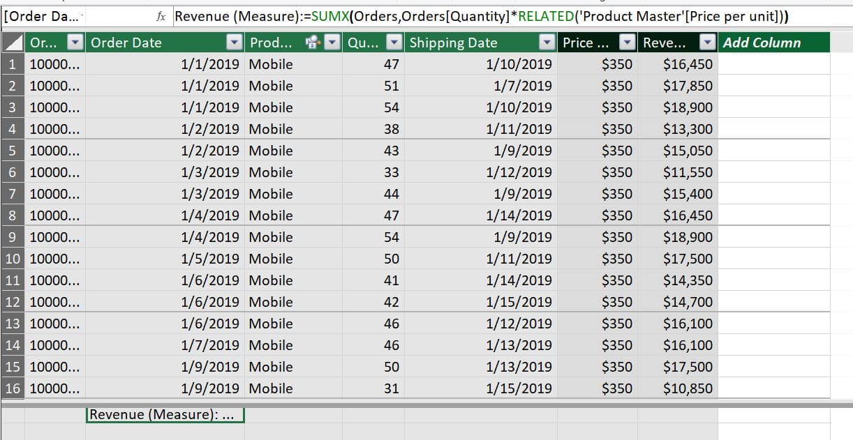
Go back to Data View and open the Orders tab. The grid of empty cells below the data is the calculation area, where measures live. Click any cell there. (If you do not see it, turn on Home → View → Calculation Area.)
Step 6: Type the measure
In the formula bar type the measure name followed by := and the formula. The practice file names the measure Revenue (Measure):
Revenue (Measure) :=
SUMX (
    Orders,
    Orders[Quantity] * RELATED ( 'Product Master'[Price per unit] )
)
Press Enter. The calculation area shows Revenue (Measure): $17,362,850. Then set the format to Currency under Home → Formatting.
In Excel 2016 and later you can also create the same measure from the Excel ribbon with Power Pivot → Measures → New Measure: choose Orders as the table, type the name and paste the formula. (This alternative is not shown in the video.)
How the formula works
- Orders – SUMX loops through every row of the Orders table that is visible in the current filter. In a PivotTable row for Laptop, that is only the Laptop orders.
- Orders[Quantity] – the quantity of the current order row.
- RELATED(‘Product Master'[Price per unit]) – follows the relationship from the current order to its product in Product Master and returns that product’s price. RELATED needs the relationship from Step 4; without it you get an error.
- The multiplication gives revenue for one order, for example 47 Mobiles × 350 = 16,450.
- SUMX adds all those order revenues together.
The column names in the formula are written with their table name, for example Orders[Quantity]. That is the recommended way to reference columns inside a measure.
Why not SUM(Quantity) × SUM(Price)?
This check is an addition, not from the video. A measure like SUM(Orders[Quantity]) * SUM('Product Master'[Price per unit]) multiplies two totals instead of multiplying row by row. At the grand total it would give 41,442 × 1,250 = 51,802,500, far from the real 17,362,850. Multiplication must happen per order and then be summed, which is exactly what SUMX does.
Part 3 – Compare with the Calculated Column
In the calculated column tutorial (LOOKUPVALUE vs RELATED) the same revenue was built with two helper columns. In the video PK recreates them quickly to compare:
Price Per Unit                = LOOKUPVALUE ( 'Product Master'[Price per unit], 'Product Master'[Product], Orders[Product] )
Revenue (Calculated column)   = Orders[Quantity] * Orders[Price Per Unit]
Then he inserts a PivotTable (Home → PivotTable in the Power Pivot window) with Product in Rows and Quantity, the calculated Revenue column and the Revenue measure in Values. Both revenue columns match exactly:
| Product | Quantity | Sum of Revenue (column) | Revenue (Measure) |
|---|---|---|---|
| Laptop | 14,091 | $8,454,600 | $8,454,600 |
| Mobile | 14,059 | $4,920,650 | $4,920,650 |
| Tablet | 13,292 | $3,987,600 | $3,987,600 |
| Grand Total | 41,442 | $17,362,850 | $17,362,850 |
The difference is where the work happens. The calculated columns store a price and a revenue on all 972 rows of the model. The measure stores nothing; it calculates the total only when a PivotTable asks for it. You only need one of the two methods; the practice file shows both side by side so you can compare.
Part 4 – Revenue by Product Pie Chart
- In the Power Pivot window open the PivotTable drop-down, choose PivotChart and place it on the existing sheet.
- Put Product on the axis and the Revenue measure in Values.
- Go to Design → Change Chart Type and pick 3-D Pie.
- Use PivotChart Analyze → Field Buttons → Hide All.
- Right-click the pie, choose 3-D Rotation and raise the Y rotation so the pie is easier to see. Delete the legend.
- Add data labels, then in Format Data Labels tick Category Name and Percentage (instead of Value) and set the position to Outside End.
The chart shows Laptop 49%, Mobile 28% and Tablet 23% of revenue.
Common Errors and Fixes
RELATED gives an error in the measure
There is no relationship between Orders and Product Master, or the Product names do not match. Create the relationship in Diagram View and make sure each product appears once in Product Master.
The measure shows the same total on every row
The field in Rows comes from a table that is not connected to Orders. Use Product from Orders or from Product Master, both of which are linked by the relationship.
Refresh fails after you download the files
This tip is an addition. The workbook remembers the folder where the text files were on PK’s computer. In the Power Pivot window go to Home → Existing Connections, edit each text connection and browse to the files on your PC.
Tips
- Use a measure for totals such as revenue, profit or cost. Use a calculated column only when you need the value on every row, for example to slice or filter by it.
- Name measures clearly, like Revenue (Measure), so they are easy to tell apart from columns in the field list.
- The same pattern works for any row-by-row total:
SUMX ( Orders, Orders[Quantity] * RELATED ( 'Product Master'[Cost] ) )would give total cost if the master had a Cost column. - Microsoft’s SUMX function reference lists the full syntax and remarks.
Want It Ready-Made?
If you want a finished Power Pivot report instead of building one, the Comparative Analysis Dashboard in Excel on NextGenTemplates.com is ready to use, and you can browse all Excel dashboard templates. To learn PivotTables, the data model and Power Pivot step by step, join the video course Excel Pivot Tables and Dashboards.
Related Tutorials
- Create Relationship in Power Pivot
- Calculated Column in Power Pivot: LOOKUPVALUE vs RELATED
- Power Pivot KPIs in Excel: Create, Edit and Delete
- Drill Down and Drill Up in a Pivot Chart with Power Pivot
Frequently Asked Questions
What does the SUMX function do in Power Pivot?
SUMX goes through a table one row at a time, evaluates an expression for each row and returns the sum of all the results. It is the DAX way to add up a calculation, such as quantity times price.
What is the difference between SUM and SUMX?
SUM adds the values of one existing column. SUMX adds the results of an expression calculated row by row, so it can combine columns, even from a related table, without a helper column.
Why do I need RELATED inside SUMX?
The price lives in Product Master, while SUMX is looping through Orders. RELATED follows the relationship from each order row to its product and returns the matching price.
Should I use a measure or a calculated column for revenue?
Both give the same totals. A measure is usually better for totals because it adds nothing to the stored data, while a calculated column is useful when you need the value on each row.
How do I create a measure in Excel 2016 or Microsoft 365?
Type it in the calculation area of the Power Pivot window, or use Power Pivot, Measures, New Measure on the Excel ribbon, pick the table, name the measure and enter the formula.
About the Author
PK is a Microsoft Excel expert and trainer and the founder of PK: An Excel Expert and NextGenTemplates.com. He has been teaching Excel, Power Pivot and Power BI since 2016 on his YouTube channel.
Conclusion
The SUMX function in Power Pivot replaces two helper columns with one measure. Import the tables, relate Orders to Product Master, and let SUMX multiply each order’s quantity by its RELATED price and add up the results. The measure returns the same $17,362,850 as the calculated columns, works in any PivotTable or chart, and keeps your model lean. Download the practice files and build the measure yourself.