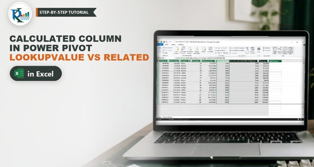
A calculated column in Power Pivot adds a new field to a data model table, computed row by row with a DAX formula. In this tutorial you have an Orders table with the quantity sold per product, and a separate Product Master text file with the price per unit. You bring the price into Orders twice, once with LOOKUPVALUE and once with RELATED, then multiply it by the quantity to get Revenue. You will see exactly when each function works, why RELATED needs a relationship, and how to build a PivotTable and chart from the result.

⬇️ Download the Calculated Column Practice File
Workbook with Power Pivot data model · .xlsx (no macros) · 972 orders plus Product Master
Watch the Video Tutorial
PK loads the Orders table and a Notepad product master into Power Pivot, adds the price with LOOKUPVALUE and RELATED, calculates Revenue, then builds the PivotTable and area chart.
What You Will Build
- A data model with an Orders table and a Product Master table imported from a text file.
- A Price Per Unit column using LOOKUPVALUE, which needs no relationship.
- The same column using RELATED, which follows a relationship between the tables.
- A Revenue column: quantity multiplied by price per unit.
- A PivotTable and area chart that refresh when the price file changes.
The Sample Data
- Orders (Excel table, 972 rows, January to August 2019): Order Id, Order Date, Product, Quantity and Shipping Date. There is no price and no revenue.
- Product Master (tab-separated text file): Product and Price per unit. Tablet 300, Mobile 350, Laptop 600.
The price sits in a Notepad file, not in the workbook, so Power Pivot imports it and looks it up inside the data model.
Part 1 – Load Both Tables into Power Pivot
Step 1: Add the Orders table to the data model
Click inside the Orders table (its name is shown on the Table Design tab). Go to Power Pivot → Add to Data Model. The Power Pivot window opens with the Orders table loaded. PK also gives Order Date and Shipping Date a short date format under Home → Formatting.
Step 2: Import the Product Master text file
- In the Power Pivot window go to Home → Get External Data → From Other Sources.
- In the Table Import Wizard scroll to the bottom, choose Text File and click Next.
- Click Browse and select Product Master.txt.
- Tick Use first row as column headers and set Column Separator to Tab. The preview now shows Product and Price per unit in two clean columns.
- Click Finish, then Close. A new Product Master tab appears at the bottom of the Power Pivot window.

Part 2 – Calculated Column in Power Pivot with LOOKUPVALUE
Step 3: Add a new calculated column
Open the Orders tab. Double-click the Add Column header, type Price Per Unit and press Enter. With the new column selected, type = in the formula bar and enter the DAX formula.
Step 4: Write the LOOKUPVALUE formula
The syntax of LOOKUPVALUE is:
LOOKUPVALUE(<result_columnName>, <search_columnName>, <search_value>
[, <search2_columnName>, <search2_value>]... [, <alternateResult>])- result_columnName – the existing column that holds the value you want back. Here:
'Product Master'[Price per unit]. It must be a column, not an expression. - search_columnName – the column to search in, in the same table as the result column or in a related table. Here:
'Product Master'[Product]. - search_value – the value to find. Here: the product of the current order row,
Orders[Product]. - alternateResult (optional) – returned when no match is found or more than one distinct result is found. Without it you get BLANK for no match and an error for more than one result.
The fully qualified formula for the Price Per Unit column is:
= LOOKUPVALUE ( 'Product Master'[Price per unit], 'Product Master'[Product], Orders[Product] )In the video and the practice file PK builds it by clicking the columns, and the formula bar shows the short form =LOOKUPVALUE('Product Master'[Price per unit],[Product],[Product]). It returns the same prices in the file, but writing the table name in front of every column makes it clear that the search happens in Product Master’s Product column for the Product of each order.
Press Enter and every order row shows its price: 300 for Tablet, 350 for Mobile and 600 for Laptop. In the video this works before any relationship exists, which is the main advantage of LOOKUPVALUE.

Part 3 – The Same Column with RELATED
Step 5: Create the relationship
RELATED only works when a relationship exists. Go to Home → View → Diagram View and drag Product from the Orders table onto Product in the Product Master table. A line joins the two tables. Orders is the “many” side and Product Master the “one” side.

Step 6: Write the RELATED formula
Back in Data View, add another column. The practice file names it Price Per Unit (RELEATED FORMULA), with the spelling as shown. The syntax has just one argument, the column you want from the related table:
RELATED(<column>)
= RELATED ( 'Product Master'[Price per unit] )
For each order row, RELATED follows the many-to-one relationship to the matching Product Master row and returns its price. The results are identical to the LOOKUPVALUE column.

What happens without the relationship?
In the video PK deletes the relationship in Diagram View (right-click the line, Delete). The RELATED column immediately shows an error, because there is no relationship to follow. Recreate the relationship and the prices come back. The LOOKUPVALUE column is not affected either way.
Part 4 – Calculate Revenue
Step 7: Add the Revenue column
Add one more column named Revenue. You can use either price column, because both hold the same values:
= Orders[Quantity] * Orders[Price Per Unit]The practice file writes it as =[Quantity]*[Price Per Unit], which is the same thing: inside a calculated column of Orders, an unqualified column name refers to the current row of Orders. The first order is 40 Tablets × 300 = 12,000.
Step 8: Format the columns
Select each price column and Revenue, then choose Home → Formatting → Data Type: Currency, the $ symbol and no decimal places.

Part 5 – Build the PivotTable and Chart
Step 9: Insert the PivotTable
In the Power Pivot window click Home → PivotTable and place it on a new worksheet. From Orders, put Product in Rows and Quantity, Price Per Unit and Revenue in Values. Price Per Unit would be summed by default, which makes no sense for a price, so open its Value Field Settings and choose Average.
| Product | Quantity | Average Price Per Unit | Revenue |
|---|---|---|---|
| Laptop | 14,091 | $600 | $8,454,600 |
| Mobile | 14,059 | $350 | $4,920,650 |
| Tablet | 13,292 | $300 | $3,987,600 |
| Grand Total | 41,442 | $419 | $17,362,850 |
Step 10: Add the area chart
In the Power Pivot window open the PivotTable drop-down and choose PivotChart, then pick Existing Worksheet and a cell below the table. Put Order Date on the axis and Revenue in Values. Use Design → Change Chart Type → Area, then PivotChart Analyze → Field Buttons → Hide All. The practice file titles it Revenue by Order Date.

Step 11: Refresh when the price changes
The model stays connected to the text file. In the video PK changes the Laptop price to 1200 in Notepad, saves it and clicks Data → Refresh All. Laptop revenue doubles to $16,909,200 and the grand total becomes $25,817,450, with no formula edits.
LOOKUPVALUE vs RELATED: Which One Should You Use?
| LOOKUPVALUE | RELATED | |
|---|---|---|
| Needs a relationship | No | Yes, many-to-one |
| Arguments | Result column, then search column and value pairs | Just the column to fetch |
| Multiple match conditions | Yes, add more search pairs | One relationship key |
| No match | BLANK, or alternateResult | BLANK |
| Best for | One-off lookups, or tables you cannot relate | A proper star-schema model |
The “multiple conditions” and “best for” rows are general DAX guidance, not shown in the video. If your tables can be related, RELATED is shorter, easier to read and is the usual choice. In the next part of this series PK skips the helper columns completely and calculates revenue with a measure, in SUMX Function in Power Pivot.
Common Errors and Fixes
RELATED shows an error
There is no relationship between the tables, or it points the wrong way. Create it in Diagram View from Orders[Product] to Product Master[Product]. RELATED always fetches from the “one” side.
LOOKUPVALUE returns an error about multiple values
The product appears more than once in Product Master with different prices. Remove the duplicate, add a second search pair, or supply an alternateResult.
The Grand Total average price looks slightly off
This is an addition beyond the video. Average of Price Per Unit is a simple average over all 972 order rows, which gives 418.52 and shows as $419. Revenue divided by quantity gives about 418.97. If you need a weighted average price, create a measure such as Avg Price := DIVIDE ( SUM ( Orders[Revenue] ), SUM ( Orders[Quantity] ) ).
Tips
- Always write the table name before a column in DAX, for example
Orders[Quantity]. It avoids confusion when two tables share a column name. - Calculated columns are stored in the model and use memory. For totals like revenue, a measure is often the leaner choice.
- Microsoft documents both functions: LOOKUPVALUE and RELATED.
Want It Ready-Made?
If you want a finished Power Pivot report instead of building one, the Comparative Analysis Dashboard in Excel on NextGenTemplates.com is ready to use, and you can browse all Excel dashboard templates. To learn PivotTables, the data model and Power Pivot step by step, join the video course Excel Pivot Tables and Dashboards.
Related Tutorials
- Create Relationship in Power Pivot
- SUMX Function in Power Pivot
- Drill Down and Drill Up in a Pivot Chart with Power Pivot
- Power Pivot KPIs in Excel: Create, Edit and Delete
Frequently Asked Questions
What is a calculated column in Power Pivot?
It is a column you add to a data model table with a DAX formula. The formula runs once for every row and the results are stored in the model, so you can use the column in PivotTables like any imported column.
What is the difference between LOOKUPVALUE and RELATED?
LOOKUPVALUE searches a column for a value and returns the matching result, with no relationship needed. RELATED fetches a value from the one side of an existing many-to-one relationship and only needs the column name.
Why does my RELATED formula return an error?
RELATED needs a relationship between the two tables. Create it in Diagram View by dragging the key column from the fact table onto the matching column in the lookup table.
Can LOOKUPVALUE match on more than one column?
Yes. Add more pairs of search column and search value after the first pair. A row is returned only when all the conditions match.
About the Author
PK is a Microsoft Excel expert and trainer and the founder of PK: An Excel Expert and NextGenTemplates.com. He has been teaching Excel, Power Pivot and Power BI since 2016 on his YouTube channel.
Conclusion
A calculated column in Power Pivot lets you enrich a table with data from anywhere in the model. LOOKUPVALUE finds the price with no relationship at all, while RELATED does the same job in one short argument once Orders and Product Master are linked. Multiply by quantity and you have Revenue, ready for a PivotTable and chart that refresh whenever the price file changes. Download the practice file and try both formulas side by side.