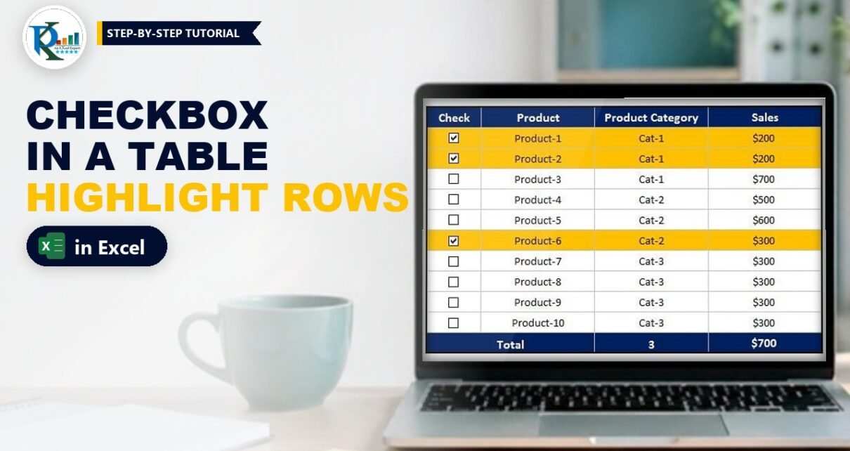
A checkbox in an Excel table is one of the quickest ways to let users pick rows. In this Excel tip you put one Form Control check box in every row of a product table. Tick a box and the whole row is highlighted, while the Total row counts the ticked products and adds up only their sales. It takes a few minutes to set up, it uses only a cell link, a conditional formatting formula, COUNTIF and SUMIF, and it needs no VBA. At the end you will also see the newer in-cell checkboxes of Microsoft 365.

⬇️ Download the Checkbox Table
.xlsx workbook (24 KB) · Excel 2010 and later for Windows · no macros
Watch the Video Tutorial
In the video, PK shows the finished table, then rebuilds it on a new sheet: one check box copied to all rows with Ctrl + D, cell links, a row-highlight rule and the COUNTIF and SUMIF totals.
What You Will Build
- A product table with a Check column, Product, Product Category and Sales.
- One check box per row, created once and copied down in a single step.
- Hidden TRUE/FALSE values under every check box.
- Row highlighting: a checked row turns gold across the whole table.
- A smart Total row that counts the checked products and sums only their sales.
How the Workbook Is Laid Out
The download has two sheets: Smart Check Box is the finished example and Sheet2 is the one PK builds in the video. Both use the same layout:
- C3:F3: headers Check, Product, Product Category and Sales.
- C4:C13: ten check boxes, each linked to the cell it sits in.
- D4:F13: Product-1 to Product-10, categories Cat-1 to Cat-3 and the sales values.
- Row 14: Total, with the count of checked products in E14 and their sales in F14.
Part 1: Set Up the Table
Step 1: Create the table
Type the four headers in C3:F3 and your data below them. Leave the Check column empty, because the check boxes will fill it. Add Total in C14, format the table with a dark header and borders, and turn off gridlines with View > Gridlines. Set the row height to about 20 so each check box has room.
Step 2: Show the Developer tab
Check boxes live on the Developer tab. If you don’t see it, go to File > Options > Customize Ribbon and tick Developer.
Part 2: Add the Checkboxes in the Excel Table
Step 3: Insert one check box
Go to Developer > Insert > Form Controls > Check Box and click in cell C4. Delete the default caption text (Check Box 1), resize the box and move it to the centre of C4. Make sure the whole control sits inside the cell.
Step 4: Copy it to every row with Ctrl + D
Select C4:C13 and press Ctrl + D (Fill Down). Excel copies C4, including the check box inside it, to every selected cell. You get ten perfectly aligned check boxes in one keystroke, which is much faster than copying and pasting them one by one.
Step 5: Link each check box to its cell
Right-click the first check box, choose Format Control and on the Control tab set Cell link to $C$4. Click OK. Repeat for every check box: the second links to $C$5, the third to $C$6, and so on down to $C$13.
A check box copied after it was linked keeps the link of the original, so give every box its own cell. Now a ticked box writes TRUE into its cell and an unticked box writes FALSE.
Step 6: Hide the TRUE and FALSE text
The words show up behind the check boxes. Select C4:C13, open Format Cells (Alt, O, E or Ctrl + 1), go to Number > Custom and type three semicolons:
;;;A custom format has sections for positive numbers, negative numbers, zero and text. Leaving all of them empty hides any value in the cell, while formulas can still read it. In the video PK first tries a white font, but the custom format is cleaner because it also works when the row is highlighted.
Part 3: Highlight Checked Rows
Step 7: Add a conditional formatting formula
Select the table body C4:F13 (start the selection in C4, so C4 is the active cell). Go to Home > Conditional Formatting > New Rule > Use a formula to determine which cells to format and enter:
=$C4Click Format, pick a fill colour on the Fill tab (the template uses gold) and click OK twice. Tick any check box and its whole row lights up.
How the formula works
- The rule is written for the active cell C4, and Excel adjusts it for every other cell in C4:F13.
- The
$before C locks the column, so every cell in a row looks at column C of that row: D7, E7 and F7 all check$C7. - The row number has no
$, so it changes from row to row. - The linked cell already holds TRUE or FALSE, so you don’t need
=$C4=TRUE. Both versions give the same result.
Part 4: Count and Sum the Checked Items
Step 8: Count checked products
In E14 enter:
=COUNTIF(C4:C13,TRUE)COUNTIF counts the cells in C4:C13 that hold TRUE, which means the checked boxes.
Step 9: Sum the sales of checked products
In F14 enter the formula below and give it the same currency format as the sales column:
=SUMIF(C4:C13,TRUE,F4:F13)SUMIF looks at the criteria range C4:C13 and adds the value from F4:F13 only where the check cell is TRUE. Tick Product-1 and Product-2 (200 each) and F14 shows $400 with a count of 2.
Modern Alternative: In-Cell Checkboxes in Microsoft 365
Addition: this section is not in the original file or video. It covers a newer Excel feature. Microsoft 365 now has native in-cell checkboxes. Instead of drawing a Form Control, you select C4:C13 and click Insert > Checkbox (in the Cell Controls group of the Insert tab). Each selected cell becomes a checkbox whose value is TRUE or FALSE, so there is no cell link to set up and nothing to hide. If you are converting the downloaded file, delete the old Form Control check boxes first.
- The same
=$C4conditional formatting rule and the same COUNTIF and SUMIF formulas work without any change. - Click the checkbox, or select the cell and press the Spacebar, to tick or untick it.
- The checkboxes move, sort and filter with their cells, which Form Controls do not always do.
- They are available in Microsoft 365 (including Excel for the web). In an Excel version without this feature, such as Excel 2021 or 2019, the cells show TRUE and FALSE instead of boxes, so keep the Form Control method for files you share with users of older versions.
Common Errors and Fixes
Ticking one box ticks all of them
The copied check boxes still share the cell link of the first one. Open Format Control for each box and give it its own cell (Step 5).
The whole table is highlighted, or only column C
The $ is in the wrong place or the selection did not start in C4. The rule must be =$C4 with C4 as the active cell when you create it.
The count and sum stay at zero
The check boxes are not linked, or they are linked to cells outside C4:C13. Tick a box and check the formula bar of its cell: it should show TRUE.
Ctrl + D did not copy the check box
The check box was not fully inside C4. Move it so it sits inside the cell borders, then select C4:C13 and press Ctrl + D again.
Tips
- Use Ctrl + click to select a Form Control check box without ticking it, then move or resize it.
- Keep the Check column narrow and centre the boxes, so they stay inside their cells when you resize rows.
- Use COUNTIF with FALSE to count the unchecked items, and divide the checked count by
ROWS(C4:C13)to show a percentage complete. - The same idea turns any list into a to-do list or a selection list for a report.
- Microsoft explains the SUMIF function with more examples on Microsoft Support.
Want It Ready-Made?
If you want ready-to-use lists with checkboxes, progress tracking and summaries, browse the Excel checklist templates on NextGenTemplates.com. To master COUNTIF, SUMIF and the other formulas behind tools like this, the Excel AI Mastery: 100 Formulas course teaches them step by step.
Related Tutorials
- Smart To-Do List with Excel’s New Checkbox Feature
- 4 Steps for Dynamic Conditional Formatting with a Check Box
- Dynamic Chart with Checkboxes in Excel
- Conditional Formatting Formula to Highlight Entire Rows
- Excel SUMIF Function with Examples
Frequently Asked Questions
How do I insert a checkbox in every row of an Excel table quickly?
Insert one Form Control check box in the first cell, remove its caption and keep it inside the cell. Then select that cell and the cells below it and press Ctrl + D. Each row gets its own aligned check box.
Why does every checkbox change together?
Copied check boxes keep the cell link of the original. Right-click each box, choose Format Control and link it to the cell it sits in.
How do I highlight a row when its checkbox is ticked?
Select the table body starting from the first check cell and add a conditional formatting rule that uses a formula pointing at the check cell with a dollar sign before the column letter, as shown in Step 7.
Can I sum only the checked items?
Yes. Use SUMIF with the check cells as the range, TRUE as the criteria and the sales column as the sum range. COUNTIF with TRUE counts the checked items.
Does this work with the new Microsoft 365 checkboxes?
Yes. In-cell checkboxes from the Insert tab store TRUE or FALSE directly in the cell, so the same highlight rule, COUNTIF and SUMIF work without any cell links.
About the Author
PK is a Microsoft Excel expert and trainer and the founder of PK: An Excel Expert and NextGenTemplates.com. He has been teaching Excel, VBA, Power Query and Power BI since 2016 on his YouTube channel.
Conclusion
A checkbox in an Excel table becomes really useful when the rest of the sheet reacts to it. Insert one Form Control check box, copy it down with Ctrl + D, link each box to its cell, hide the TRUE/FALSE with a custom format, highlight rows with a simple formula rule and total the checked items with COUNTIF and SUMIF. On Microsoft 365, the in-cell checkboxes make the same setup even faster. Download the file and try it with your own list.