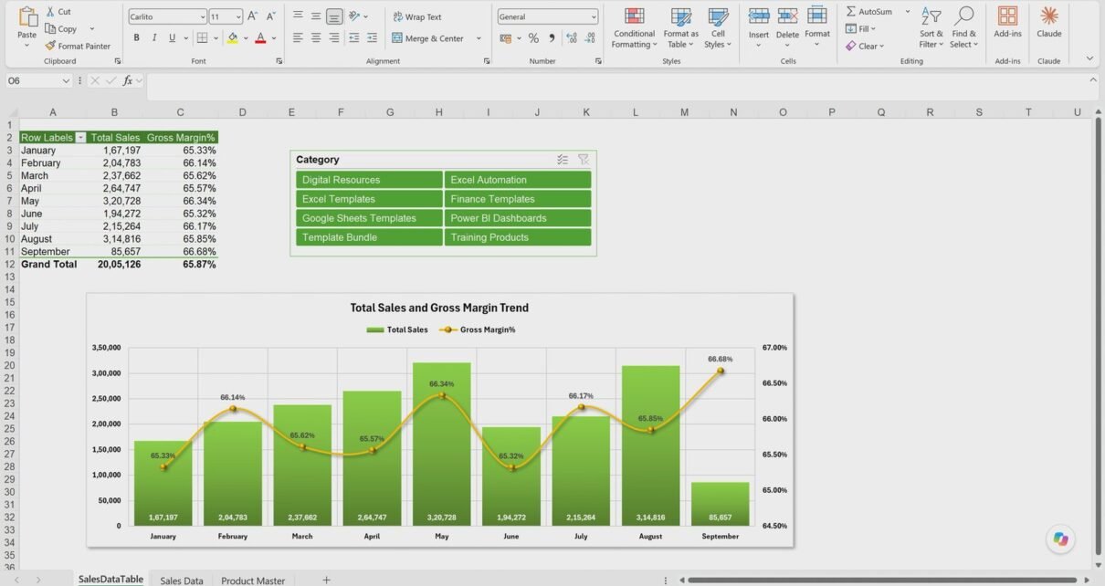
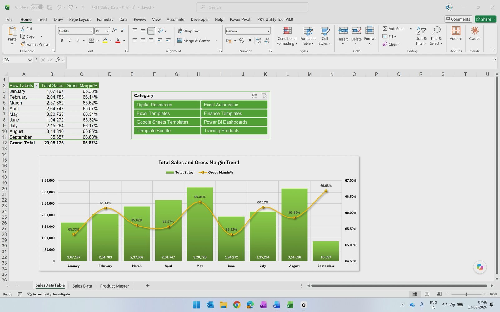
Merge queries in Power Query in Excel to combine two tables in a few clicks instead of writing VLOOKUP formulas. In this tutorial we merge a 350-row Sales Data table with a 25-product Product Master on Product code, add Total Cost, Total Sales and Gross Margin columns, and turn the result into a monthly PivotTable report. The finished report shows 2,005,126 in total sales at a 65.87% gross margin, filtered by 8 product categories with a slicer.
If you keep sales transactions in one sheet and product details such as cost and price in another, you normally need a VLOOKUP for every column you want to bring across. Power Query does the same job with one merge step that refreshes automatically, and you can load the result straight into a PivotTable without helper formulas.
📥 Download the free practice file (start file + solution): Merge Queries in Power Query Excel Practice File
Watch the Video Tutorial
Video Overview
In this 14-minute video, PK starts with two normal ranges and converts them to tables named SalesDataTable and ProductMasterData. He loads the sales table to Power Query, changes the Date column to Date only, and adds the Product Master query by editing the Source step to Excel.CurrentWorkbook(). He then uses Home › Merge Queries to join both tables on Product code (350 of 350 rows matched), expands the product columns without the column-name prefix, and adds Total Cost, Total Sales and Gross Margin with the Standard Multiply and Subtract commands. After adding Year and Month name columns, he loads the query to a PivotTable, creates a Gross Margin % calculated field, builds a combo chart with the margin line on a secondary axis, and finishes with a Category slicer. Use the chapters in the video description to jump to any step.
What You Will Build
- 📊 A Sales Data table (Date, Product code, Unit sold) merged with a Product Master table (Product name, Category, Cost per unit, Price per unit).
- 🧮 Three calculated columns in Power Query: Total Cost, Total Sales and Gross Margin.
- 📅 Year and Month name columns for monthly reporting.
- 📈 A PivotTable with a Gross Margin % calculated field, a Total Sales and Gross Margin trend combo chart, and a Category slicer.
The Sample Data
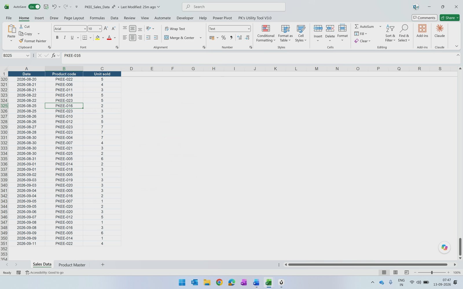
The workbook has two normal ranges. The Sales Data sheet records the units sold by product code and date, from 1 January 2026 to 11 September 2026.
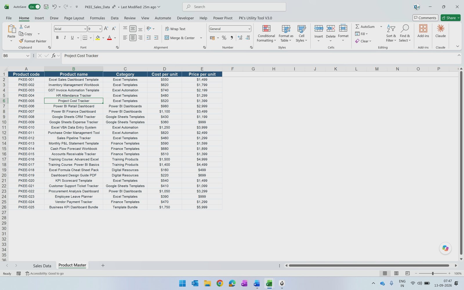
The Product Master sheet lists every product once with its name, category, cost per unit and price per unit. Product code is the common column in both tables.
Step 1: Convert Both Ranges to Excel Tables
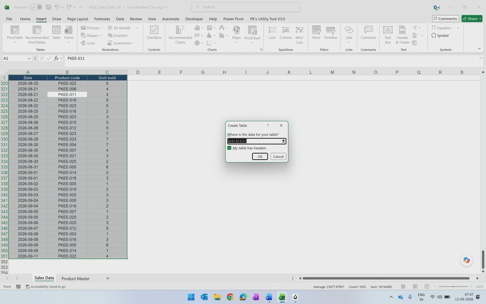
Click anywhere inside the Sales Data range and go to Insert › Table, or press Ctrl + T. Keep My table has headers ticked and click OK.
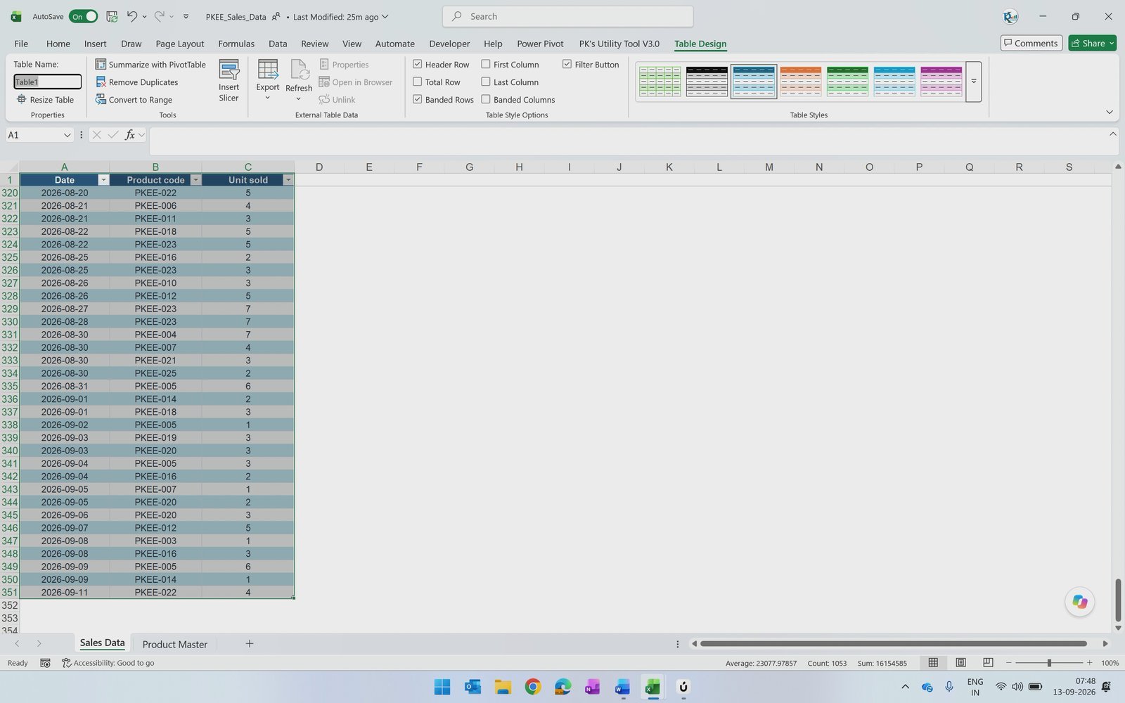
On the Table Design tab, rename the table to SalesDataTable. Repeat for the Product Master range and name it ProductMasterData. You can also untick Banded Rows for a cleaner look. Clear table names make the queries easier to read later.
Step 2: Load the Sales Data to Power Query
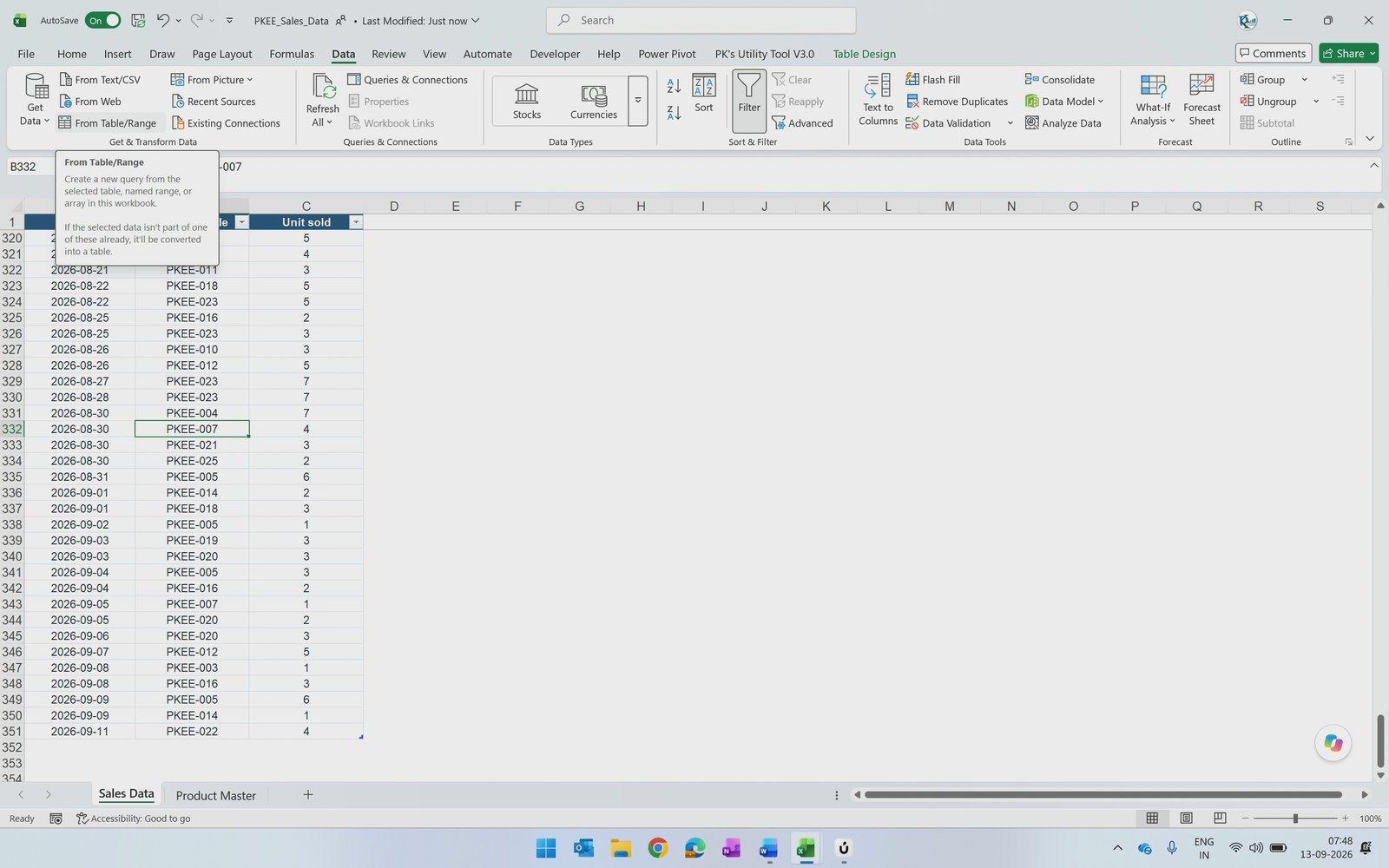
Click inside SalesDataTable and go to Data › From Table/Range. The same command is also available under Get Data › From Other Sources › From Table/Range.
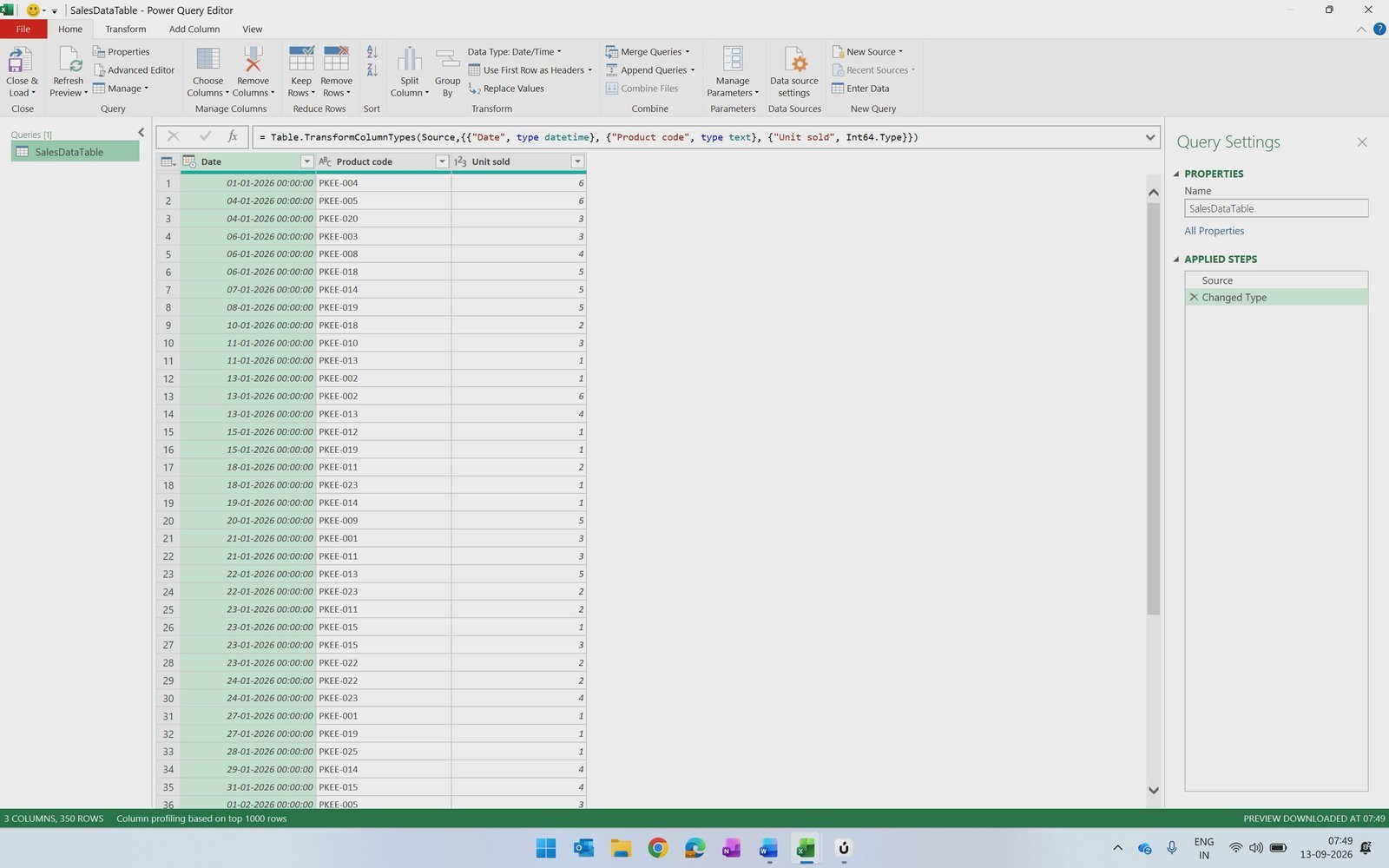
The Power Query Editor opens with the full sales table loaded.
Step 3: Change the Date Column to Date Only
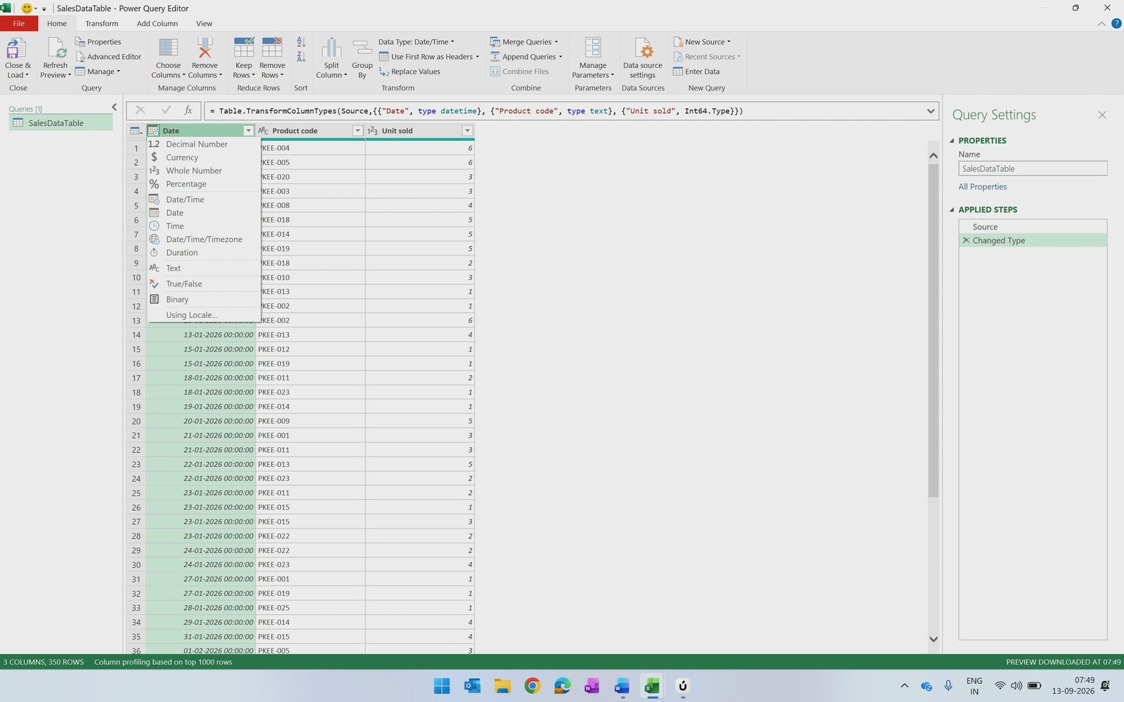
The Date column comes in as Date/Time. Click the data type icon in the Date column header and choose Date.
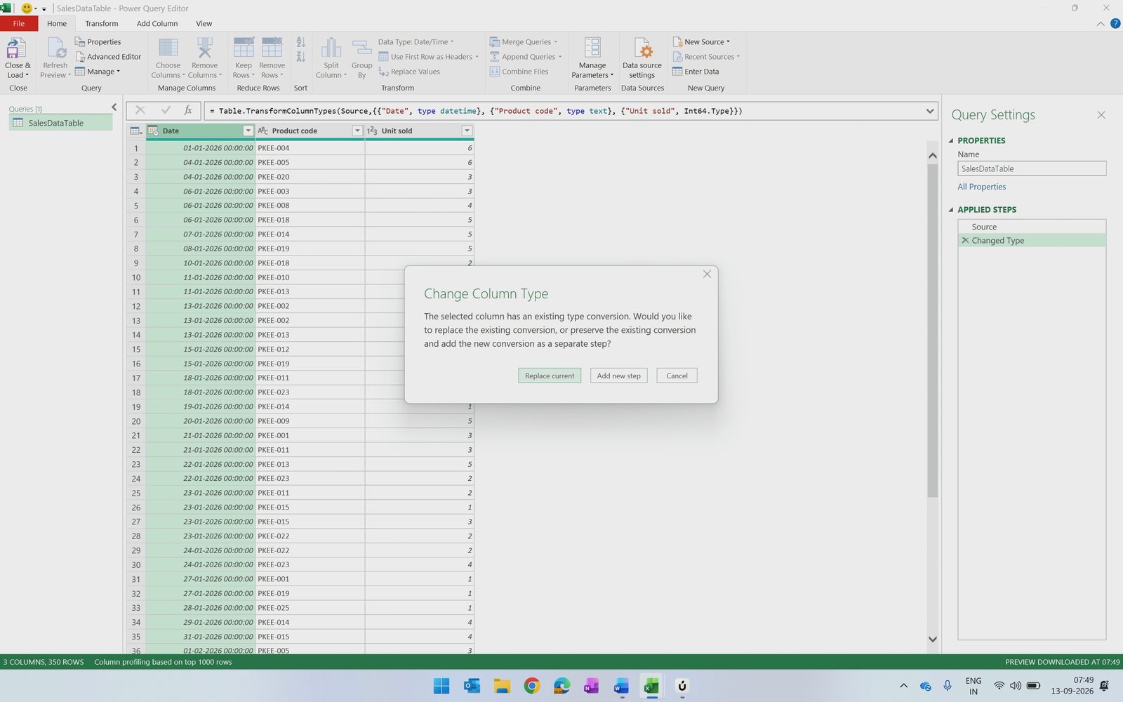
When Power Query asks whether to replace the existing conversion, click Replace current so you do not add an extra step.
Step 4: Add the Product Master Query with Excel.CurrentWorkbook()
You also need the Product Master table in Power Query. A quick way is to duplicate the SalesDataTable query, delete its Changed Type step and keep only the Source step.
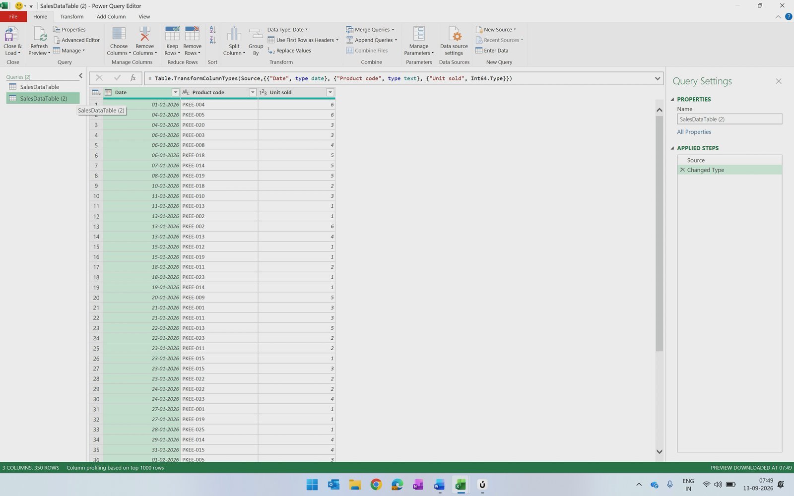
Look at the Source formula. It points to the sales table by name:
= Excel.CurrentWorkbook(){[Name="SalesDataTable"]}[Content]
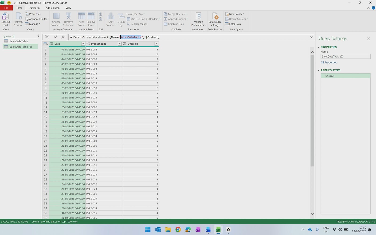
You could type the other table name here. If you do not remember the exact name, delete everything after the brackets so the formula reads = Excel.CurrentWorkbook() and press Enter.
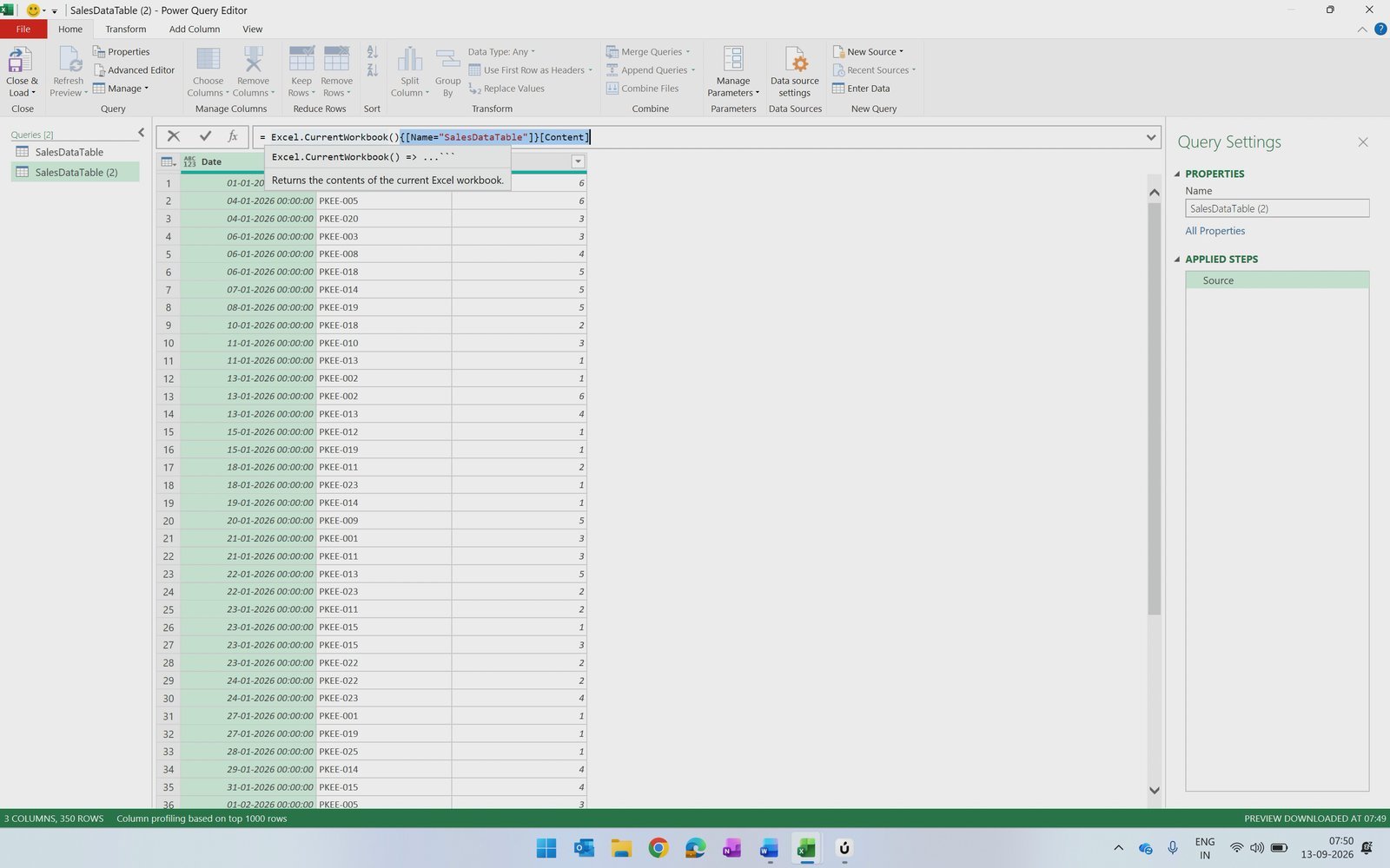
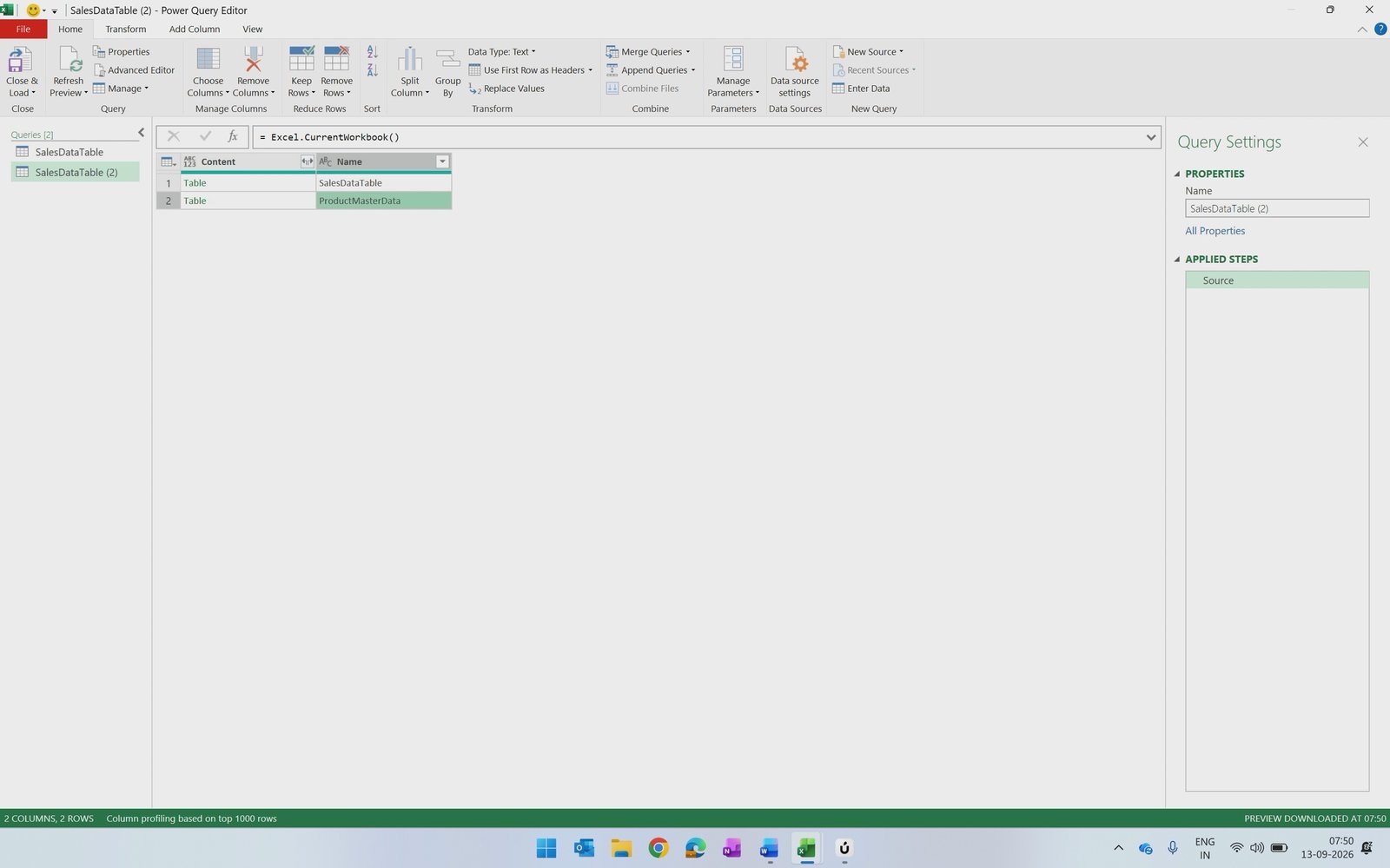
Power Query now lists every table in the workbook. Click Table next to ProductMasterData; a Navigation step is added automatically. Rename the query to ProductMasterData so the two queries are easy to tell apart.
Step 5: Merge Queries on Product Code
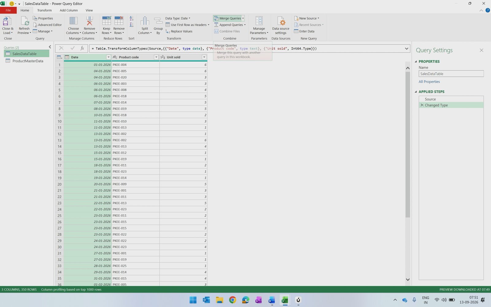
Select the SalesDataTable query and click Home › Merge Queries. Merge Queries as New would create a third query; here we bring the product columns directly into the sales query.
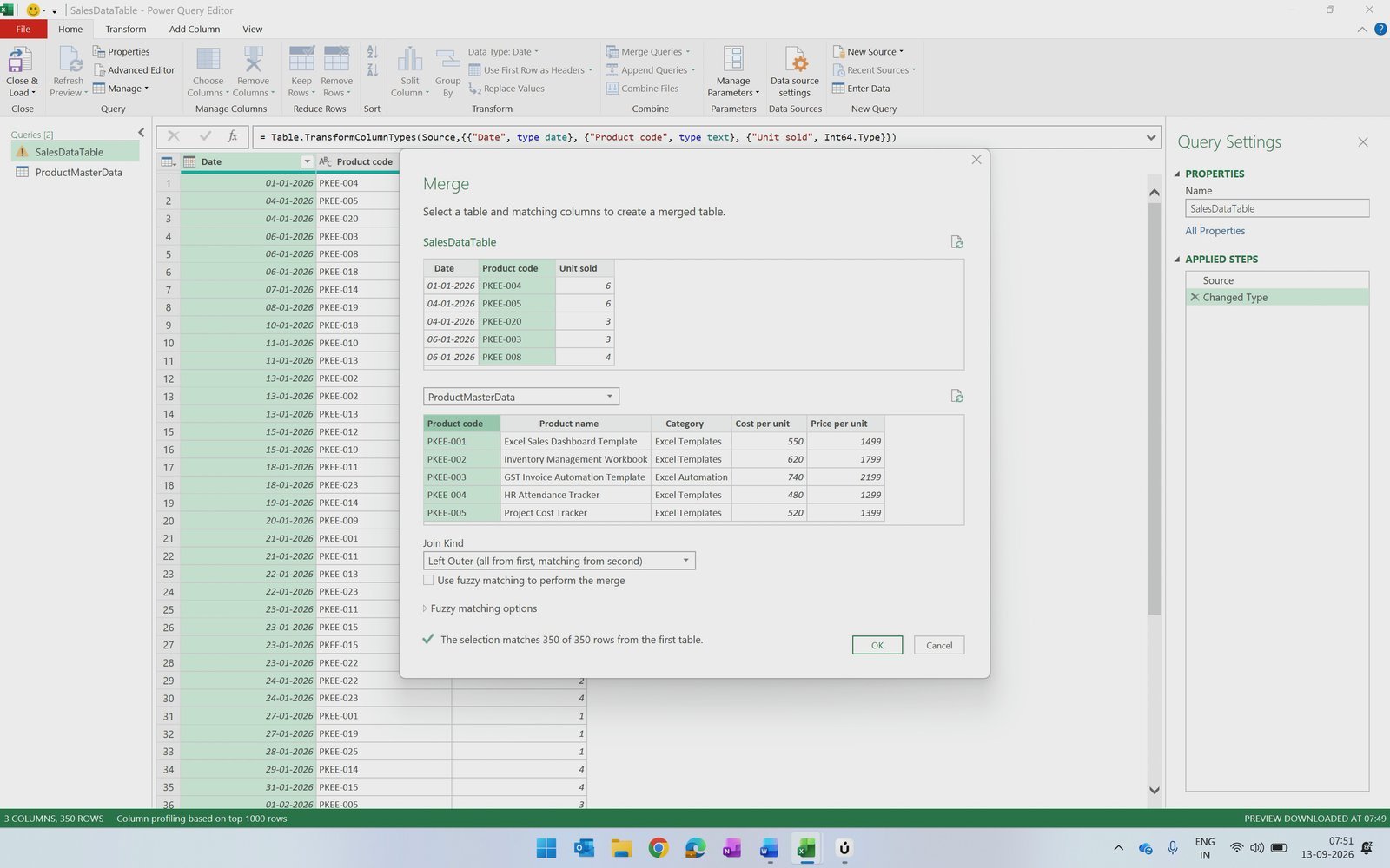
In the Merge dialog, choose ProductMasterData as the second table. Click the Product code column in both tables and keep the Join Kind as Left Outer (all from first, matching from second). The status line at the bottom confirms the selection matches 350 of 350 rows from the first table. Click OK.
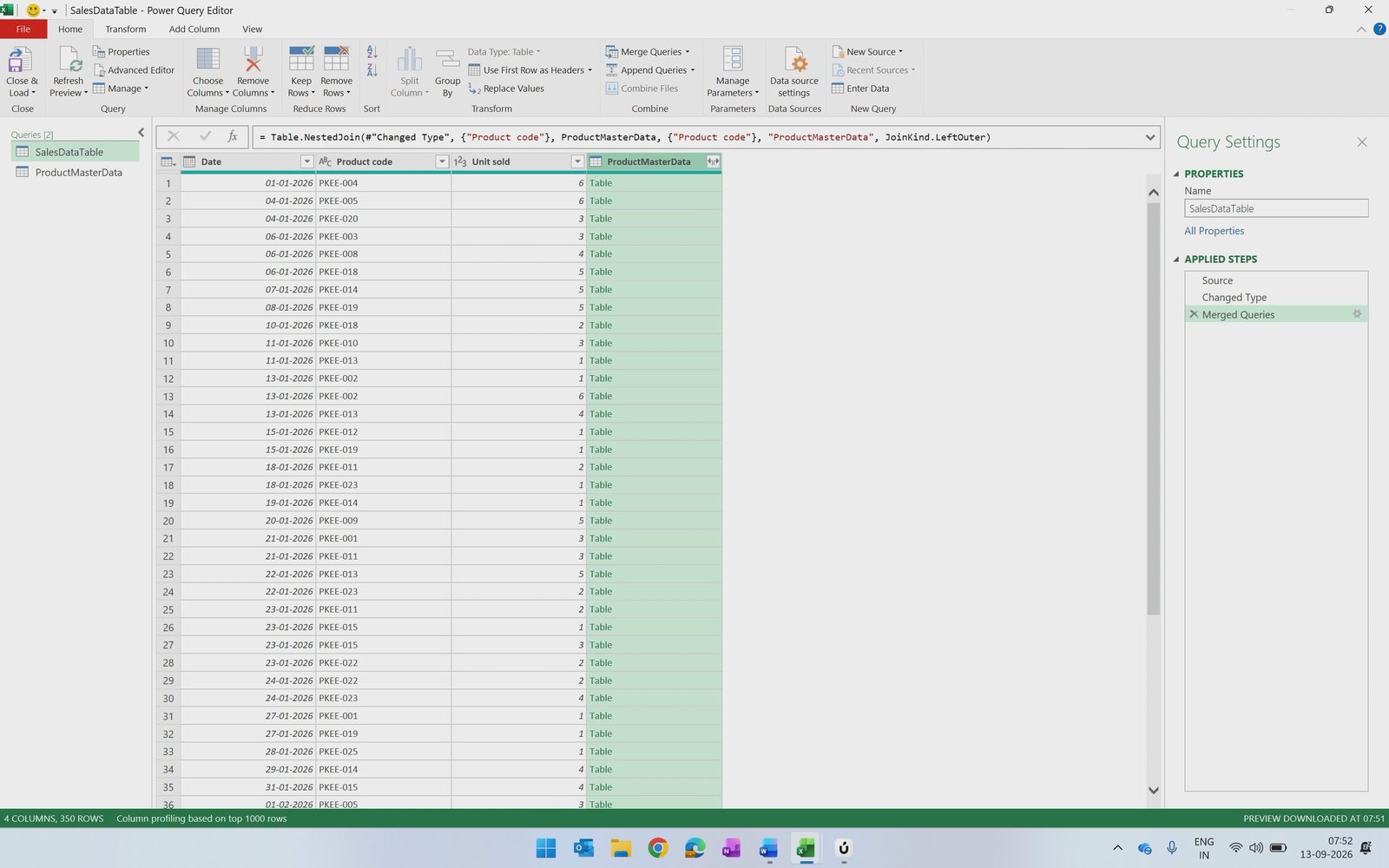
A new column named ProductMasterData appears, holding a small table for each row. Click any cell in it to preview the matching product record.
Step 6: Expand the Product Master Columns
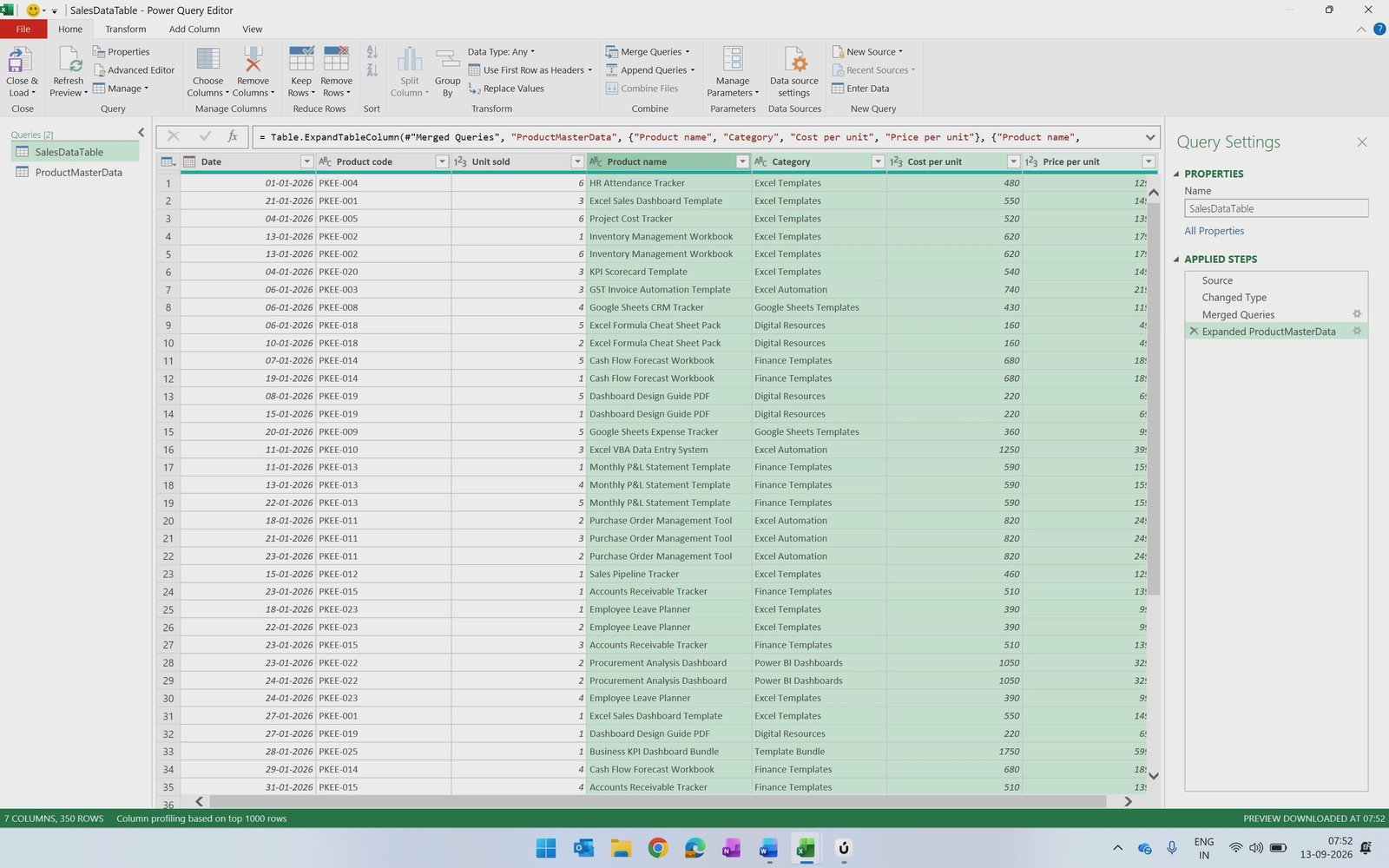
Click the two-headed arrow in the ProductMasterData column header. Untick Product code, because it is already in the sales table, and untick Use original column name as prefix so the new columns keep clean names. Click OK.
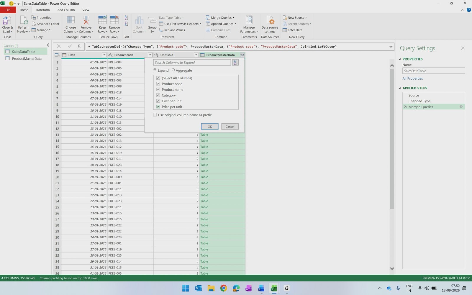
Product name, Category, Cost per unit and Price per unit now sit next to every sales row, all in one table.
Step 7: Add Total Cost and Total Sales Columns
Select Unit sold, hold Ctrl and click Cost per unit. Go to Add Column › Standard › Multiply.
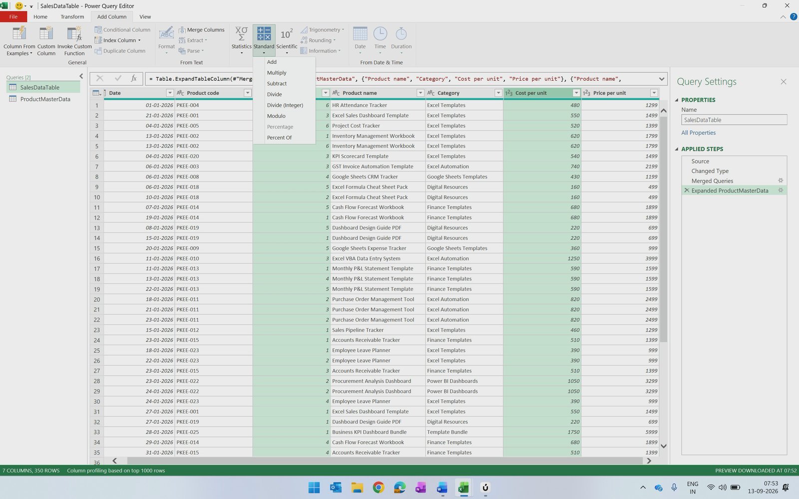
Power Query writes the formula for you. You never need to edit it, but it is worth reading:
= Table.AddColumn(#"Expanded ProductMasterData", "Multiplication", each [Unit sold] * [Cost per unit], Int64.Type)
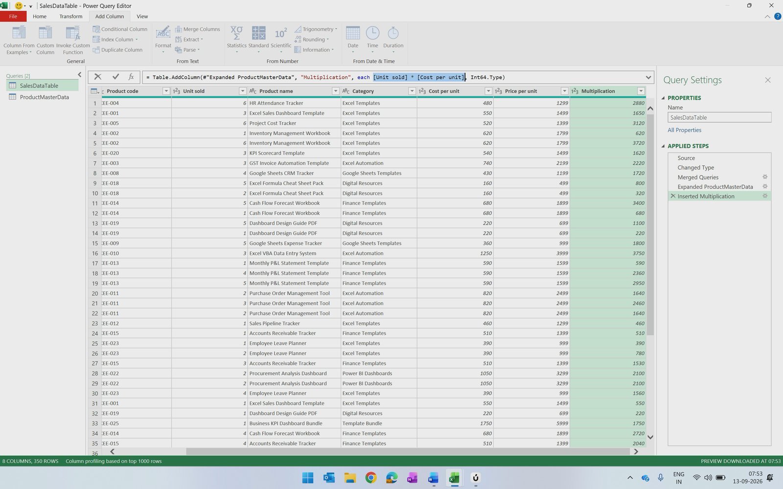
Rename the new column to Total Cost. Repeat with Price per unit and Unit sold to create Total Sales.
Step 8: Calculate Gross Margin
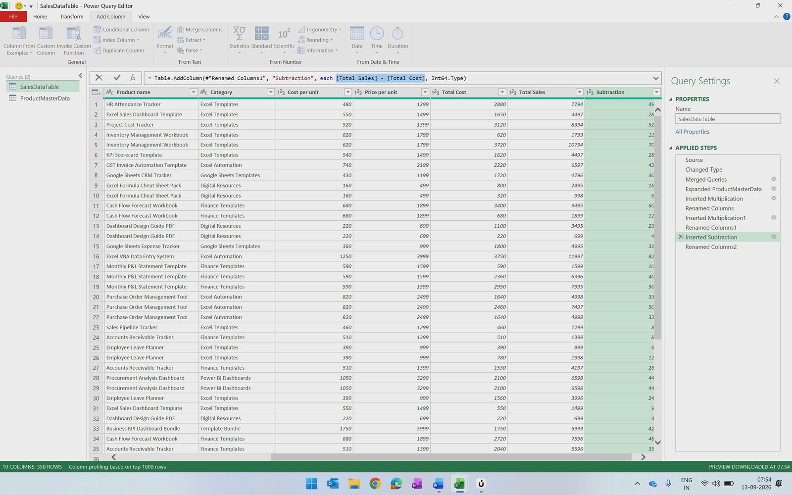
Gross Margin = Total Sales − Total Cost. The order of selection matters: click Total Sales first, then Ctrl + click Total Cost, and go to Add Column › Standard › Subtract.
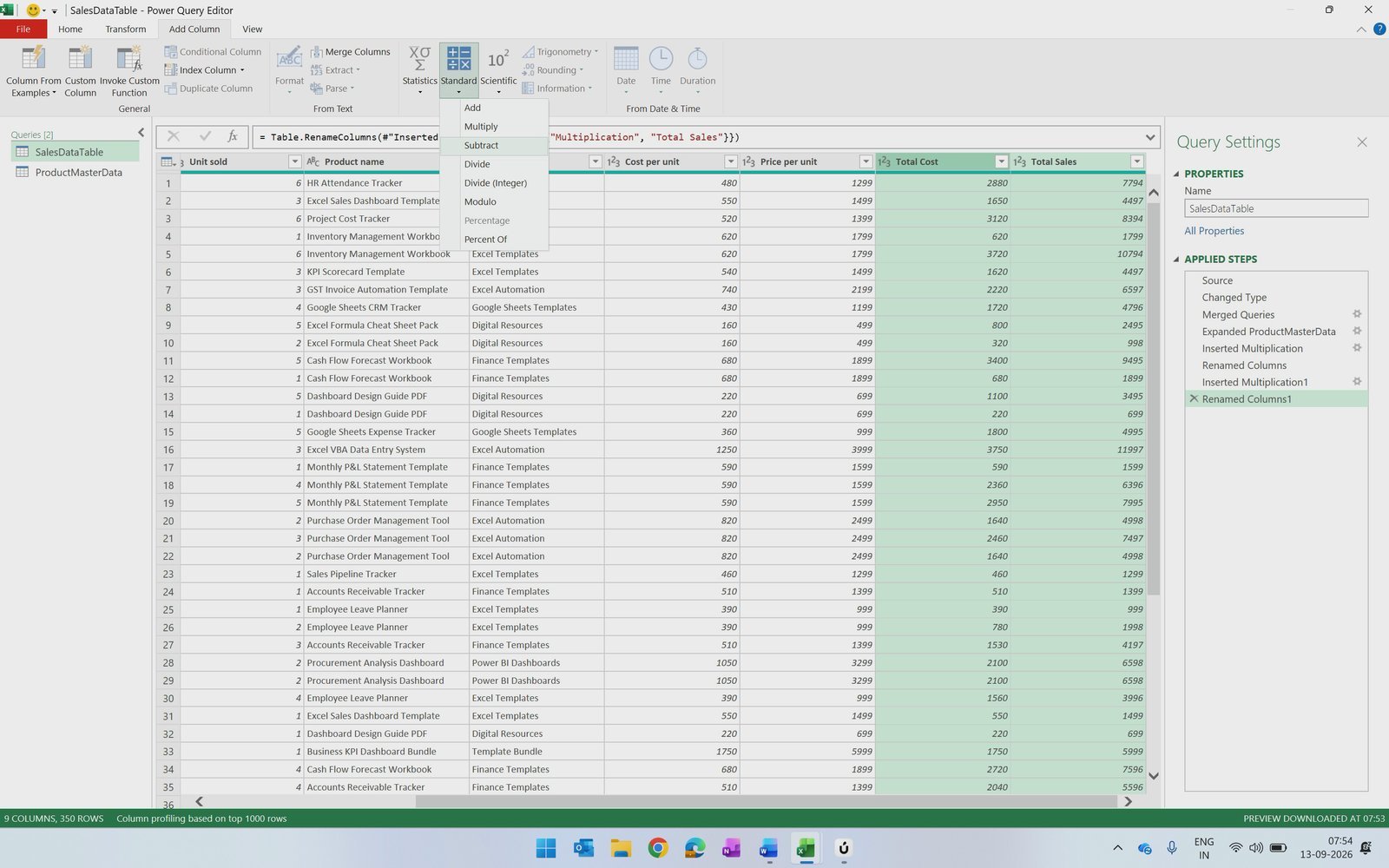
Rename the column to Gross Margin, then click the previous step and check the formula. It must read [Total Sales] - [Total Cost], not the other way round.
Step 9: Close & Load to a PivotTable
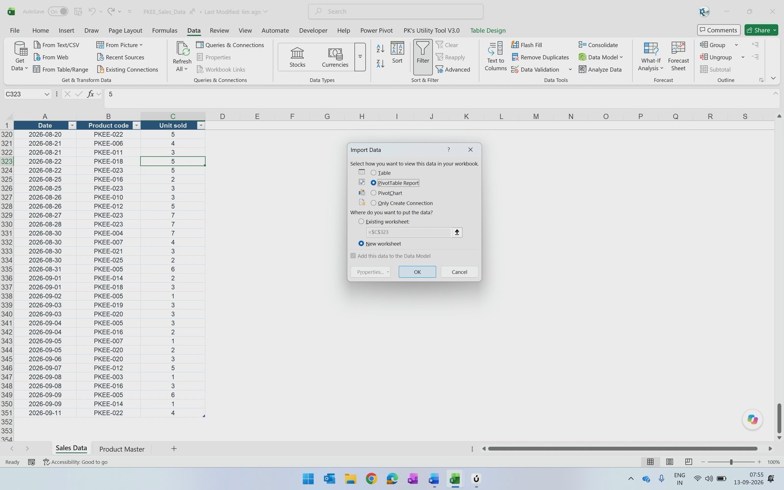
Click Home › Close & Load To. In the Import Data dialog choose PivotTable Report and New worksheet. If you pick Only Create Connection, nothing is loaded to the sheet, but the query stays available under Data › Queries & Connections.
Step 10: Add Year and Month Columns
To report by month, reopen the editor with Data › Get Data › Launch Power Query Editor. Select the Date column and choose Add Column › Date › Year › Year, then Add Column › Date › Month › Name of Month.
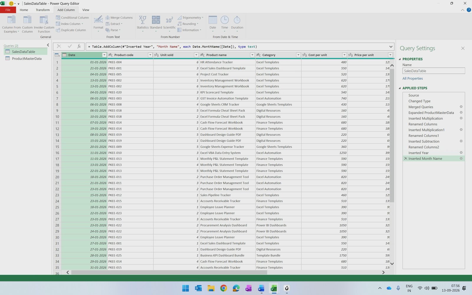
Click Close & Load. The query refreshes and the new columns are available to the PivotTable. If you need a fresh PivotTable, right-click the query in Queries & Connections and use Load To › PivotTable Report.
Step 11: Create a Gross Margin % Calculated Field
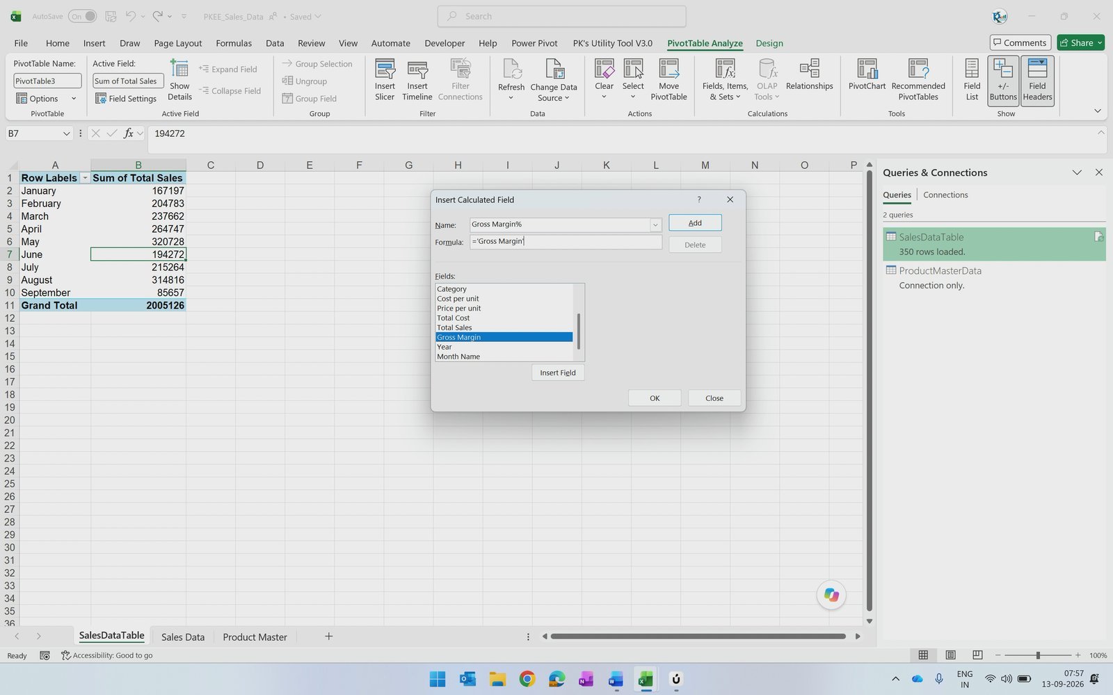
Put the month name in Rows and Total Sales in Values. The data has Gross Margin as an amount but not as a percentage, so click inside the PivotTable and go to PivotTable Analyze › Fields, Items & Sets › Calculated Field.
Name the field Gross Margin% and use the formula = 'Gross Margin' / 'Total Sales'. Click OK, then set the value field’s number format to Percentage.
Step 12: Build the Combo Chart
Go to Insert › Recommended Charts › All Charts › Combo. Keep Sum of Total Sales as a clustered column, set Gross Margin% to Line with Markers and tick Secondary Axis.
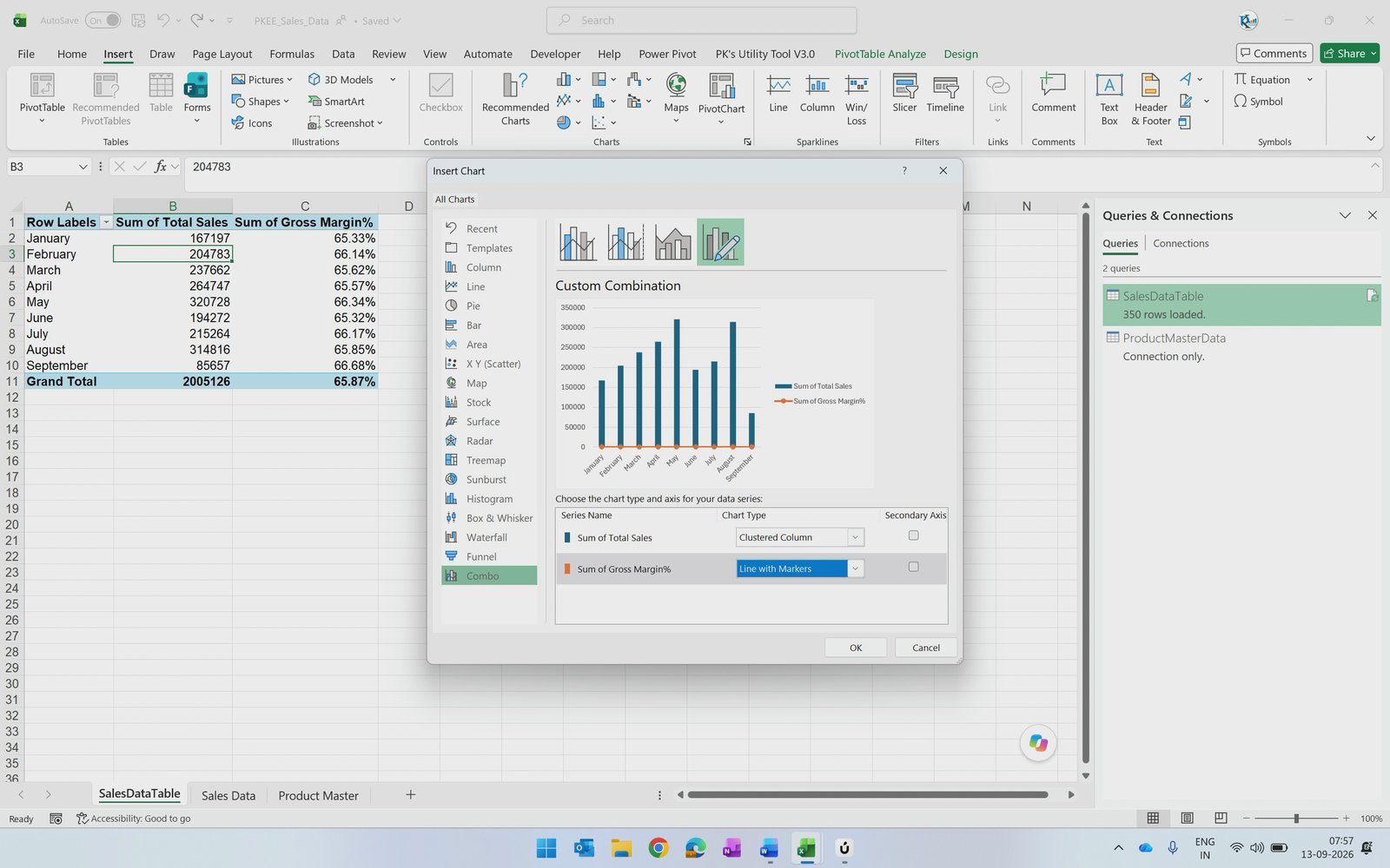
A few formatting touches make the chart presentation-ready:
- Rename the value fields to remove “Sum of”. Add one space before the name (for example
Total Sales), because a PivotTable field cannot have exactly the same name as a source column. - Add a chart title such as Sales and Margin Trend, hide the field buttons (PivotChart Analyze › Field Buttons) and move the legend to the top.
- Give the columns a gradient fill with a gap width of about 20%, and make the line smooth with 6 pt markers.
- Add data labels: above the line points, and inside base in white for the columns so they stay readable.
Step 13: Add a Category Slicer
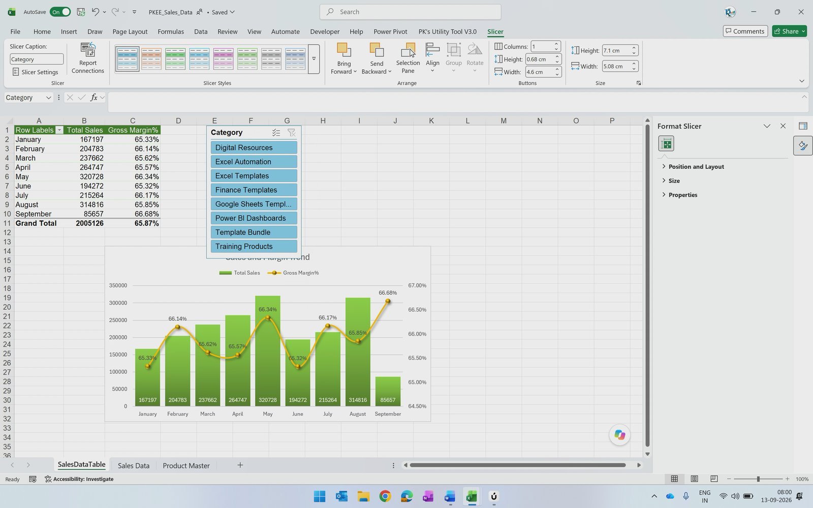
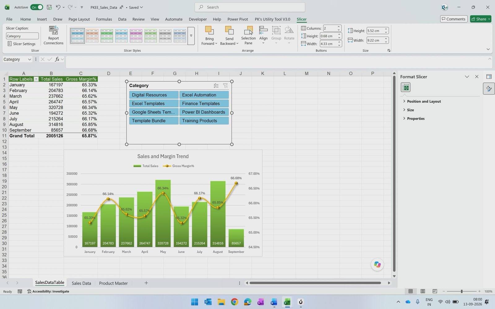
Select the PivotTable and choose Insert › Slicer › Category. Set the slicer to two columns, resize it and pick a slicer style. Clicking a category now filters the PivotTable and the chart together.
Merge Queries vs. VLOOKUP vs. XLOOKUP
| Feature | Power Query Merge Queries | VLOOKUP | XLOOKUP |
|---|---|---|---|
| Columns brought across in one step | ✅ All selected columns at once | One formula per column | One formula (spill) per lookup |
| Refresh when data grows | ✅ Refresh All | Copy formulas down | Copy formulas down |
| Formulas stored in the sheet | ✅ None | Yes | Yes |
| Join types (left, inner, anti) | ✅ Six join kinds | Left match only | Left match only |
| Match check | ✅ Shows matched rows (350 of 350) | #N/A errors | #N/A or custom text |
| Load straight to a PivotTable | ✅ Yes | No | No |
| Excel versions | Excel 2016 and later, Microsoft 365 | All versions | Excel 2021, Microsoft 365 |
| Learning curve | Medium | Low | Low |
For recurring reports where the sales data grows every month, merging queries in Power Query replaces dozens of lookup formulas with one refreshable step.
Tips and Best Practices
- ✅ Always convert source ranges to named tables before loading them; the names appear in the Excel.CurrentWorkbook() list.
- ✅ Check the match count in the Merge dialog. Anything less than all rows means some product codes are missing or spelled differently.
- ✅ Fix data types (such as Date) before merging and adding columns.
- ✅ For subtraction and division, select the columns in the order the formula needs, then verify the step formula.
- ✅ Keep calculations in Power Query and ratios in the PivotTable: a margin % must be calculated from totals, not summed row by row.
Want to go further? Read Mastering Merged Query & PIVOT Column Techniques in Power Query and Dynamic Pivot Table with Multiple Tables using Power Query. You can also compare approaches in Attendance Sheet in Excel: 7 Methods Compared. Microsoft’s official Merge queries overview explains every join kind in detail.
Short on time? Browse ready-made Excel Dashboard Templates and Excel KPI Dashboards on NextGenTemplates.
Frequently Asked Questions
What does Merge Queries do in Power Query?
Merge Queries in Power Query joins two tables on one or more matching columns, similar to a database join. In this Excel tutorial it adds Product name, Category, Cost per unit and Price per unit from the Product Master table to every sales row by matching Product code.
Is merging queries in Power Query better than VLOOKUP?
For reports that refresh regularly, yes. Merge Queries brings several columns across in one step, stores no formulas in the sheet and updates with Refresh All, while VLOOKUP needs one formula per column that must be copied down whenever the data grows.
What is the difference between Merge Queries and Merge Queries as New?
Merge Queries adds the joined columns to the query you have selected, which keeps the workbook to two queries. Merge Queries as New leaves both source queries unchanged and creates a third query that contains the merged result.
Which join kind should I use to merge two tables in Excel?
Use Left Outer when you want every row from the first table, such as all sales transactions, plus matching details from the second table. Power Query also offers Right Outer, Full Outer, Inner, Left Anti and Right Anti joins for other scenarios.
Why do I remove the column name prefix when expanding a merged table?
By default Power Query names expanded columns like ProductMasterData.Category. Unticking Use original column name as prefix keeps the original names, such as Category and Cost per unit, which makes the table and the PivotTable fields easier to read.
How do I calculate gross margin percentage from a Power Query table?
Add Total Sales, Total Cost and Gross Margin columns in Power Query, load the query to a PivotTable, and create a calculated field with the formula Gross Margin divided by Total Sales. Format it as a percentage so the ratio is calculated from totals.
Which Excel versions support Power Query merge queries?
Power Query is built into Excel 2016, Excel 2019, Excel 2021 and Microsoft 365 under Data › Get & Transform Data. Excel 2010 and 2013 users can install the free Power Query add-in from Microsoft.
Download the Free Practice File
Practice every step with the same data used in this tutorial. The download includes a start file with the Sales Data and Product Master ranges and a completed solution workbook.
👉 Click here to download the Merge Queries in Power Query practice file
About the Author
Written by PK, Microsoft Certified Professional with over 16 years of cross-industry experience in Excel, VBA, Power Query and Power BI, and the creator of the PK: An Excel Expert YouTube channel with 300K+ subscribers. Every tutorial comes with a practice file and a step-by-step video.
Conclusion
Merging queries in Power Query turns two separate tables into one analysis-ready table without a single VLOOKUP. Once the merge, calculated columns and PivotTable are in place, you only need to add new sales rows and click Refresh All to update the whole report.
🎥 Watch more tutorials on our YouTube channel: Youtube.com/@PK-AnExcelExpert
📅 Last updated: September 2026