KPI in Power Pivot for dashboard and report

Key performance indicators (KPIs) are visual measures of performance. Based on a specific calculated field, a KPI is designed to help users quickly evaluate the current value and status of a metric against a defined target. The KPI gauges the performance of the value, defined by a Base measure (also known as a calculated field in Power Pivot in Excel 2013), against a Target value, also defined by a measure or by an absolute value. If your model has no measures, see Create a measure.

Table of Contents

Create a KPI

In Data View, click the table that has the measure that will serve as the Base measure. If you have not already created a base measure.
Make sure the Calculation Area is displayed in Power pivot data model window. If it is not showing, in Power Pivot data model window, click Home>> Calculation Area.
The Calculation Area appears beneath the table in which you are currently in.
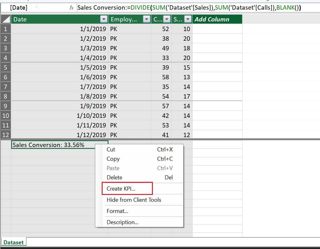
In the Calculation Area, right-click the calculated field that will serve as the base measure (value), and then click Create KPI.

You can create the KPI from Power Pivot tab also available in excel ribbon.

Go to the Power Pivot tab in your Excel ribbon >> Click on KPI >> Choose New KPI

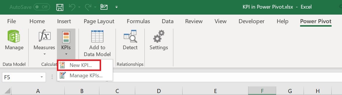
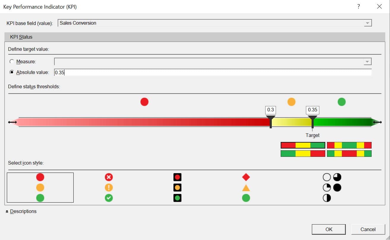
Create KPI from Power Pivot tab in Excel Ribbon

KPI window will be popped up.
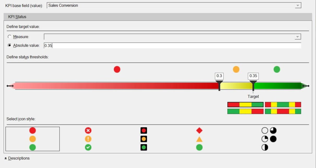
In Define target value, select from one of the following:
Select Measure, and then select a target measure in the box. Make sure you have created the measure for Target.
Select Absolute value, and then type a numerical value.
In Define status thresholds, click and slide the low and high threshold values.
In Select icon style, click an image type.
Click Descriptions, and then type descriptions for KPI, Value, Status, and Target.

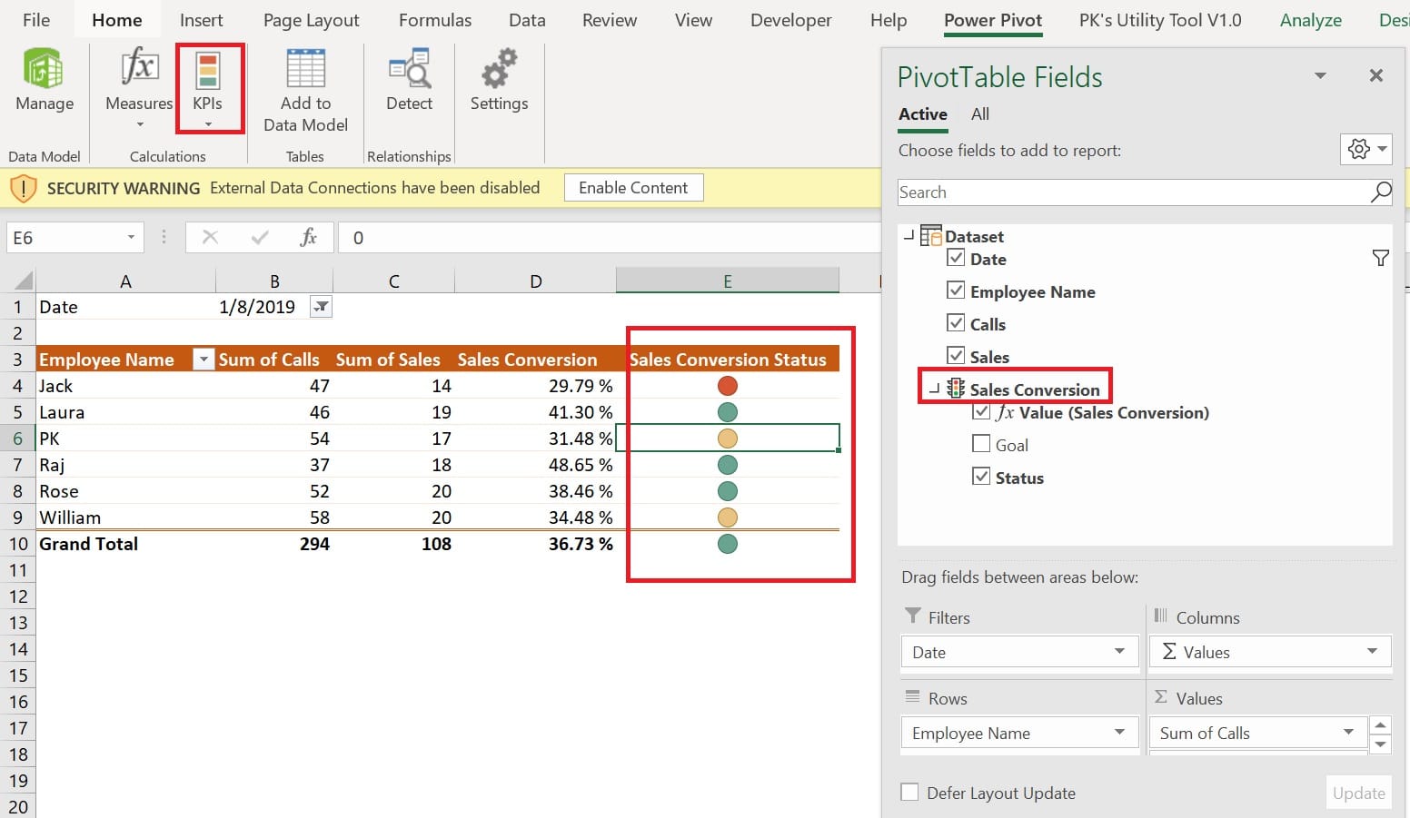
You can display the KPI in the pivot table. Create a pivot table form data model. In the Pivot Table fields window you will see a KPI icon against the base measure.

Edit a KPI

In the Calculation Area, right-click the measure that serves as the base measure (value) of the KPI, and then click Edit KPI Settings.

Delete a KPI

In the Calculation Area, right-click the measure that serves as the base measure (value) of the KPI, and then click Delete KPI.
Deleting a KPI does not delete the base measure or target measure (if one was defined)