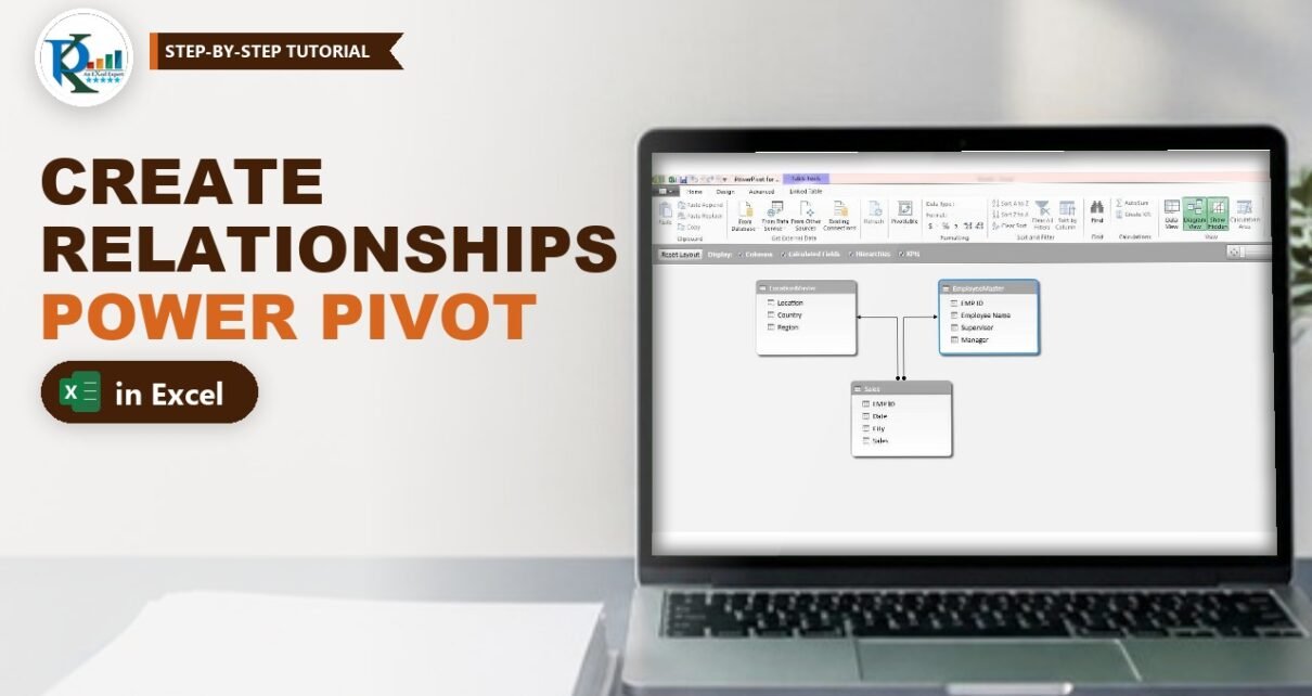
To create a relationship in Power Pivot, you add each table to the Excel Data Model and then link a column in one table to the matching column in another, usually by dragging one onto the other in Diagram View. In this tutorial you connect one fact table (Sales) to two dimension tables (Location Master and Employee Master), then build a single PivotTable that shows sales by country and by manager, even though the Sales sheet contains neither. No VLOOKUP columns, no helper formulas, and the workbook stays fast.
⬇️ Download the Practice File
Workbook with Data Model · .xlsx (no macros) · Excel 2013 and later for Windows
Watch the Video Tutorial
In the video PK turns three ranges into tables, adds them to the Data Model, drags the matching columns together in Diagram View and builds two PivotTables and a PivotChart from all three tables at once.
What You Will Build
- Three Excel tables: Sales, LocationMaster and EmployeeMaster.
- A Data Model that holds all three tables inside the workbook.
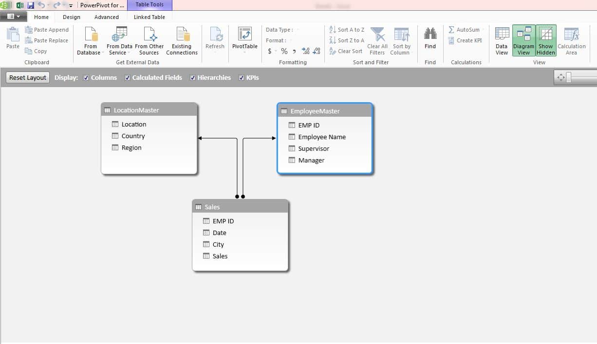
- Two relationships: Sales City to LocationMaster Location, and Sales EMP ID to EmployeeMaster EMP ID.
- A PivotTable by Manager, Supervisor and Employee in tabular form.
- A PivotTable by Region, Country and Location, plus a country PivotChart filtered by manager.
The Practice Data: One Fact Table and Two Dimension Tables
The workbook has three data sheets:
- Sales (fact table): 5,420 rows from 1 January to 28 September 2019 with EMP ID, Date, City and Sales. This is where the numbers live.
- Location Master (dimension table): 19 rows with Location, Country and Region, for example Jaipur, India, Asia & Pacific.
- Employee Master (dimension table): 20 rows with EMP ID, Employee Name, Supervisor and Manager.
The Sales sheet has no Country, Region or Manager column. The classic fix is a VLOOKUP column for each of them, but on thousands of rows those formulas recalculate constantly and slow the file down. A relationship does the same job inside the Data Model without a single formula on the sheet.
A relationship needs one column in each table that holds matching values. Here City in Sales matches Location in Location Master, and EMP ID appears in both Sales and Employee Master. In the dimension tables those values must be unique: every city and every employee ID appears only once.
Step 1: Turn On Power Pivot
In Excel 2016 and later for Windows, including Microsoft 365, Power Pivot is built in. If you do not see the Power Pivot tab, go to File → Options → Add-ins, choose COM Add-ins in the Manage box, click Go and tick Microsoft Power Pivot for Excel. In the video, which uses Excel 2013, PK opens the same list from Developer → COM Add-ins and ticks Microsoft Office PowerPivot for Excel 2013.
Step 2: Convert Each Range into a Named Table
Click inside the Sales data and press Ctrl+T (or Ctrl+L). Keep My table has headers ticked and click OK. Repeat for Location Master and Employee Master.
Then give each table a clear name in Table Design → Table Name: Sales, LocationMaster and EmployeeMaster. As PK points out, table names cannot contain spaces, so remove them. Good names make the Diagram View and the PivotTable field list much easier to read.
Step 3: Add the Tables to the Data Model
Select a cell in the Sales table and click Power Pivot → Add to Data Model. The Power Pivot window opens with a Sales tab. Close or minimise it, go back to Excel and do the same for LocationMaster and EmployeeMaster. When you are done, the Power Pivot window shows three tabs, one per table.
Step 4: Create the Relationships in Diagram View
Open Diagram View
In the Power Pivot window click Home → Diagram View. Each table appears as a box with its column names. Sales is the fact table; LocationMaster and EmployeeMaster are the dimension tables around it.
Link City to Location
Drag Location from the LocationMaster box and drop it onto City in the Sales box. A line appears between the two tables. Hover over the line and Power Pivot highlights the two columns it connects.
Link EMP ID to EMP ID
Drag EMP ID from EmployeeMaster onto EMP ID in Sales. Now all three tables are related, and the diagram looks like the screenshot above.
Power Pivot works out the direction for you: the dimension table is the one side, because each city or employee appears once there, and Sales is the many side, because the same city appears on many sales rows.
Alternative: the Create Relationship dialog
This method is an addition; the video uses drag and drop. In the Power Pivot window you can also use Design → Create Relationship, pick the Sales table and its City column, then pick LocationMaster and its Location column, and click OK. Outside the Power Pivot window, Data → Relationships → New in Excel opens a similar dialog. All three methods create the same relationship.
Step 5: Build a PivotTable from All Three Tables
Insert the PivotTable
In the Power Pivot window click PivotTable and choose New Worksheet. The PivotTable Fields list now shows all three tables.
Sales by country, filtered by manager
Tick Sales from the Sales table, then drag Country from LocationMaster into Rows. You get sales by country even though the Sales sheet has no Country column; the relationship looks it up for you. With the practice data, India leads with 143,276, followed by Vietnam with 30,309.
Insert a column PivotChart from it if you like, and drag Manager from EmployeeMaster into Filters. Pick Manager-1 or Manager-2 and the chart redraws for that manager’s team. One PivotTable is now using fields from all three tables.
Step 6: Format the Two Summary Reports
Manager, Supervisor and Employee
Clear the fields and put Manager, Supervisor and Employee Name in Rows, with Sum of Sales in Values. Then use PivotTable Design → Report Layout → Show in Tabular Form so each level gets its own column, choose a PivotTable style, and untick View → Gridlines for a clean look. The totals in the file are 135,603 for Manager-1 and 135,237 for Manager-2.
Region, Country and Location
Copy the PivotTable, paste it beside the first one and swap the fields for Region, Country and Location from LocationMaster. Both reports end at the same grand total of 270,840, which is a quick check that every sales row found its match.
Common Errors and Fixes
Relationships between tables may be needed
The PivotTable shows this yellow message when you use fields from two tables that are not related. The numbers repeat the same total on every row. Create the missing relationship and refresh.
Power Pivot will not create the relationship
One side must have unique values. If the dimension table has a duplicate city or employee ID, remove it. Also make sure both columns have the same data type, for example both whole numbers for EMP ID.
Some sales land in a blank row
A city in Sales has no match in Location Master, often because of a spelling difference or a trailing space. Add the missing city to the master table or clean the text, then refresh.
Tips
- Keep dimension tables small and clean: one row per city, product or employee.
- Name tables before adding them to the Data Model; renaming later is possible but messier.
- Use Update All on the Power Pivot tab after you add rows to the Excel tables.
- Once tables are related, the DAX
RELATEDfunction can bring a dimension value into the fact table as a calculated column. - Microsoft’s article on creating a relationship between tables in Excel covers the dialog method in more detail.
Want It Ready-Made?
To see Power Pivot relationships used in finished tools, look at the Dynamic Attendance Sheet Using Power Pivot or the KANBAN Board with Power Pivot and VBA on NextGenTemplates.com, or browse more Excel report templates. To go further with Power Pivot, PivotTables and dashboards, take the course Excel Pivot Tables and Dashboards on NextGenTemplates Academy.
Related Tutorials
- Calculated Column in Power Pivot: LOOKUPVALUE vs RELATED
- SUMX Function in Power Pivot
- Power Pivot KPIs in Excel: Create, Edit and Delete
- Combine Tables into a Dynamic PivotTable with Power Query
- Excel Comparative Analysis Dashboard with Power Pivot
Frequently Asked Questions
What is a relationship in Power Pivot?
It is a link between a column in one table and a matching column in another table of the Data Model. It lets one PivotTable use fields from both tables, much like a lookup but without formulas on the sheet.
What is the difference between a fact table and a dimension table?
The fact table holds the transactions and numbers, such as the Sales sheet. Dimension tables describe them, such as Location Master and Employee Master, with one row per city or employee.
Do I need Power Pivot to create a relationship?
No. In Excel 2013 and later you can also use Data, Relationships, New. Power Pivot adds the Diagram View, which makes larger models easier to see and manage.
Why do I need unique values in the master table?
Power Pivot relationships are one-to-many. The master table is the one side, so each key such as a city or EMP ID must appear only once there.
Can I still use VLOOKUP instead?
Yes, but each lookup adds a formula column to every row. With thousands of rows and several lookups, a Data Model relationship is faster and easier to maintain.
About the Author
PK is a Microsoft Excel expert and trainer and the founder of PK: An Excel Expert and NextGenTemplates.com. He has been teaching Excel, Power Query and Power BI since 2016 on his YouTube channel.
Conclusion
To create a relationship in Power Pivot, turn each range into a named table, add all three to the Data Model, and drag the matching columns together in Diagram View: Location onto City and EMP ID onto EMP ID. From then on one PivotTable can report sales by region, country, manager or employee straight from the Sales table, with no VLOOKUP columns at all. Start with the practice file and then try the same model on your own data.