Test Tube Chart in Excel: Thermometer KPI Chart Step by Step

Part of the free Module 9: Advanced Charts and Infographics · Lesson 3 of 8 · Full Excel course

Updated on 5 September 2026 · Works in Excel 365, 2021, 2019 and 2016 unless noted.

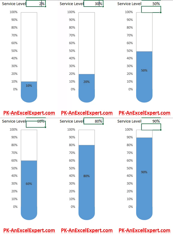
A test tube chart in Excel, also called a thermometer chart, shows a single KPI such as service level or target attainment as a coloured liquid level rising inside a narrow tube with a rounded base. You build it from a two-series stacked column chart with a fixed axis and one Flowchart: Delay shape. This lesson builds the tube from a blank sheet and links it to a cell so the level moves automatically.

How a test tube chart works

The tube is a stacked column with two values: the KPI and its remainder to 100 percent. The remainder is set to No fill with a grey border, so only the KPI portion appears filled, and the vertical axis is fixed from 0 to 1 so the level is always proportional. A rotated Delay shape placed under the chart forms the rounded bottom.

Test tube charts are compact, so several can sit side by side to compare teams, sites or months on a dashboard. The steps work in Excel 2013 through Microsoft 365 and need no VBA.

The support data explained

Cell	Entry	Purpose
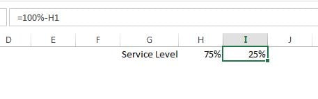
G1	Service Level	Metric name, used as the series name
H1	75%	The KPI; link it to your data or type a value
I1	=100%-H1	Empty part of the tube, drawn with No fill

Because H1 and I1 always total 100 percent, the column keeps the same height and only the filled portion changes. The fixed axis in Step 3 guarantees this even if a value is temporarily blank.

Step 1: set up the data

1. In G1 type the metric name (Service Level).
2. In H1 enter the metric value, for example 75%.
3. In I1 enter =100%-H1 for the empty part of the tube.

Step 2: insert and shape the column

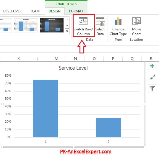
1. Select H1:I1 and go to Insert > Charts > Insert Column or Bar Chart > 2-D Column > Stacked Column.

2. On the Chart Design tab (Design under Chart Tools in Excel 2016 and 2019) click Switch Row/Column so both values stack in one column.

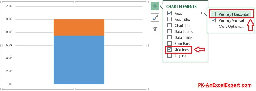
3. Click the plus sign beside the chart, untick Axes > Primary Horizontal and untick Gridlines.

4. Select the chart area, open the Format tab and set the chart Width to about 1.2 inches (3 cm) so the column becomes a narrow tube.

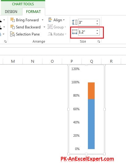
5. Right-click the column and choose Format Data Series.

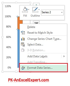
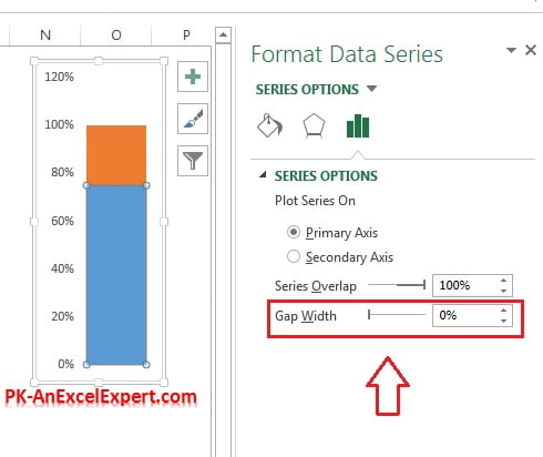
6. Set Gap Width to 0% so the column fills the plot area.

Step 3: fix the axis and colour the tube

1. Right-click the vertical axis and choose Format Axis.

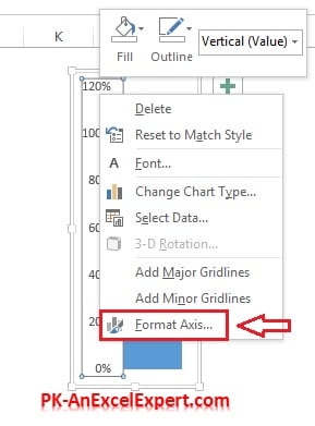
2. Under Axis Options type 0 for Minimum, 1 for Maximum and 0.1 for Major units. Type the values even if they already show, so they change from Auto to Reset and stay fixed when the KPI changes.

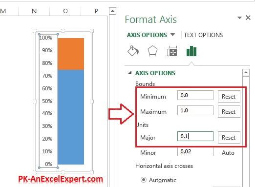
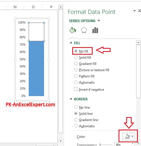
3. Double-click the remainder segment (orange) and set its fill to No fill with a grey Border. This is the empty part of the tube.

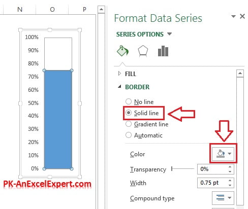
4. Double-click the KPI segment (blue) and give it the same grey border so the tube outline is continuous.

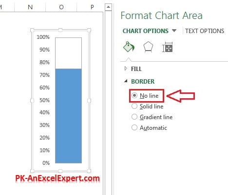
5. Select the whole chart and set its Border to No line.

Step 4: add the rounded base and the label

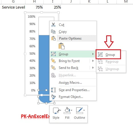
1. Go to Insert > Shapes and choose Flowchart: Delay.

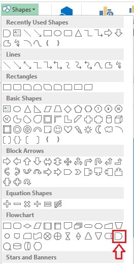
2. Select the shape and choose Format > Rotate > Rotate Right 90 degrees so the rounded side points down.

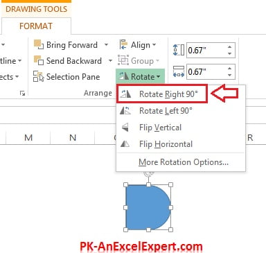
3. Choose Format > Shape Outline > No Outline and give the shape the same fill colour as the KPI segment.

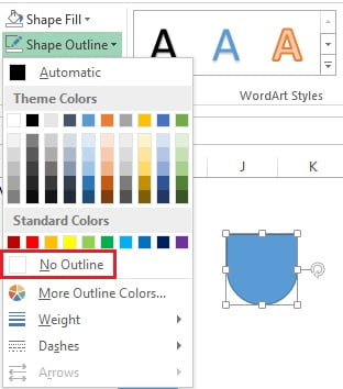
4. Resize the shape to the tube width and place it directly under the chart so the join is invisible.

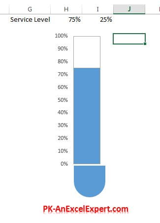
5. Select the shape and the chart together (Ctrl+click) and press Ctrl+G to group them.

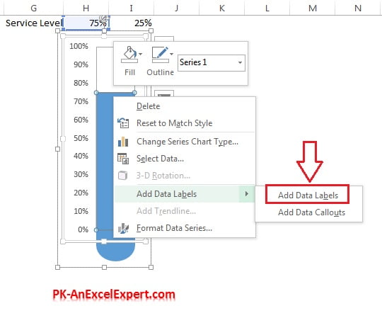
6. Right-click the KPI segment and choose Add Data Labels so the percentage shows inside the tube.

Worked example: three tubes for three teams

A quality manager wants to compare three teams in one chart. Type this table in G1:J2 and use row 3 for the remainders.

	Team A	Team B	Team C
Quality score	92%	78%	64%
Remainder	=100%-H2	=100%-I2	=100%-J2

1. Select G1:J3 and insert a Stacked Column chart. Do not click Switch Row/Column this time; each team is a category.
2. Fix the axis at 0 to 1, set Gap Width to about 80 percent, and format the remainder series with No fill and a grey border.
3. Insert three Delay shapes, rotate them, and place one under each column. Group everything.

Result: three tubes side by side showing 92, 78 and 64 percent, with the same scale so the reader can compare at a glance.

Download the practice file and video

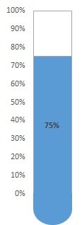
Download the Test Tube Chart Excel file to compare with your build, or click the chart below.

When to use a test tube chart

• Percentage KPIs with a natural 100 percent ceiling: service level, quality score, fundraising progress, target attainment.
• Several tubes in a row to compare teams, sites or months in a compact space.
• Not for values above 100 percent or negative values; use a column chart for those.

Tips and common mistakes

• Fix the axis before hiding it. On Auto the tube rescales when the KPI changes, so a 50 percent value can look full.
• Match the base width. Keep the Delay shape exactly as wide as the plot area, or the join shows.
• Cap the input. Wrap the KPI in MIN(H1,100%) so the fill cannot exceed the tube.
• Group before copying. If you copy the chart alone, the base is left behind.
• Add a liquid effect. Give the fill a gradient that is darker at the bottom.
• Add a target line. Insert a thin rectangle at the target height and group it with the chart, or add a third series plotted as a line.
• Use a readable label. A white, bold data label works best on a dark fill; set the chart area to No fill so the tube sits cleanly on a coloured dashboard.

Practice exercise

1. Build the single tube with 75 percent, then test 10, 50 and 100 percent to confirm the tube height never changes.
2. Build the three-team version from the worked example and add data labels to all three.
3. Make the fill turn red below 70 percent by splitting the KPI into two series with IF formulas, as in the battery chart lesson.
4. Add a small text box above the tube linked to the metric name in G1.

Key takeaways

• A test tube chart is a two-series stacked column: KPI plus remainder to 100 percent.
• Fix the vertical axis from 0 to 1 so the fill level is always proportional.
• The empty part is No fill with a grey border; the chart border is removed.
• A rotated Flowchart: Delay shape forms the rounded base; group it with the chart.
• Skip Switch Row/Column to get several tubes in one chart.

Related lessons

• Advanced Charts and Infographics course hub
• Battery chart in Excel
• Progress circle chart in Excel
• Bullet chart in Excel
• Stacked column chart basics
• Infographic thermometer chart (blog post with download)
• Microsoft Support: Create a chart from start to finish

Frequently asked questions

Is a test tube chart the same as a thermometer chart?

Yes. Both are a two-series stacked column with a fixed 0 to 100 percent axis and a rounded base shape. The name depends on the styling: a thermometer usually has a bulb at the bottom and tick marks, while a test tube has a plain rounded base. The build steps are identical.

Why does the tube rescale when I change the value?

The vertical axis is still on Auto. Open Format Axis and type 0 for Minimum and 1 for Maximum so they switch to Reset. Excel then keeps the scale fixed and only the filled portion changes. Do this before you hide the axis, because you cannot format an axis that has been removed.

Can I build several tubes in one chart?

Yes. Put each KPI and its remainder in a separate column, insert a stacked column chart without Switch Row/Column and add a Delay shape under each column. Every tube shares the same fixed axis, which makes the comparison honest.

How do I add a target marker to the tube?

Add a third series holding the target value, then use Change Chart Type to plot it as a Line with Markers on the same axis. Hide the line, keep a wide dash marker, and it sits at the target height. A simpler option is a thin rectangle shape grouped with the chart.

Does the test tube chart work in Excel for the web?

The chart itself displays and updates in Excel for the web, and stacked column formatting is available there. Shape rotation and grouping are limited in the browser, so build the base shape in desktop Excel and the file will look the same when opened online.

Want the finished version? Ready-made Excel thermometer charts, dashboards and KPI templates are available at NextGenTemplates.com.