Advanced Filter in Excel: Criteria Range and Unique Records

Part of the free Module 4: Sort and Filter · Lesson 6 of 11 · Full Excel course

Updated on 5 September 2026 · Works in Excel 365, 2021, 2019 and 2016 unless noted.

Advanced Filter in Excel filters a list using conditions typed into worksheet cells called a criteria range. Unlike AutoFilter it accepts any number of conditions, combines AND and OR logic across columns, uses formulas as criteria, copies the matching rows to another location and extracts unique records. You find it under Data > Sort & Filter > Advanced in every desktop version of Excel.

What Advanced Filter does that AutoFilter cannot

AutoFilter is fast, but each column accepts at most two conditions, it only filters in place, and the conditions disappear when you clear the filter. Advanced Filter reads its rules from cells, so you can document them, edit them, reuse them and even drive them with formulas. It also writes results to a new range, which is how analysts built report extracts and de-duplicated lists for years before the FILTER and UNIQUE functions arrived in Excel 365.

How to set up a criteria range

The criteria range is a small block of cells, usually placed above the data or on its own sheet. The first row holds column headers copied exactly from the list. Each row below holds the conditions. Three rules govern everything:

• Same row = AND. Every condition on one row must be true for a record to pass.
• Different rows = OR. A record passes if it satisfies any one row.
• A blank cell means no condition for that column on that row, and a completely blank row matches every record.

Text criteria match the beginning of the cell, so Sup matches Supervisor-1 and Supervisor-2. Use the comparison operators =, <>, >, <, >= and <= for numbers, dates and text. Wildcards work too: ? for one character, * for any run of characters and ~ before a wildcard to treat it literally. The table shows the layouts you will use most often, based on a list with the headers Location, Supervisor and Sales.

Goal	Criteria range layout	Logic
Supervisor-1 only	Supervisor in the header cell, Supervisor-1 beneath it	Single condition
Supervisor-1 with Sales above 10	Headers Supervisor and Sales; one row with Supervisor-1 and >10	AND
Supervisor-1 or any sale above 10	Same headers; row 1 has Supervisor-1 and a blank, row 2 has a blank and >10	OR
Supervisor-1 with Sales above 10, or anything in Pune	Headers Location, Supervisor, Sales; row 1 blank, Supervisor-1, >10; row 2 Pune, blank, blank	Mixed
Sales between 5 and 10	Header Sales twice; one row with >=5 and <=10	AND on one column
Everything except Delhi	Location header, <>Delhi beneath	Not equal
Locations starting with M	Location header, M* beneath	Wildcard
Exactly “Delhi”, not “Delhi North”	Location header, ="=Delhi" beneath	Exact match
Sales above the average	Blank header, =D2>AVERAGE($D$2:$D$100) beneath	Formula criteria

How to filter by a single field

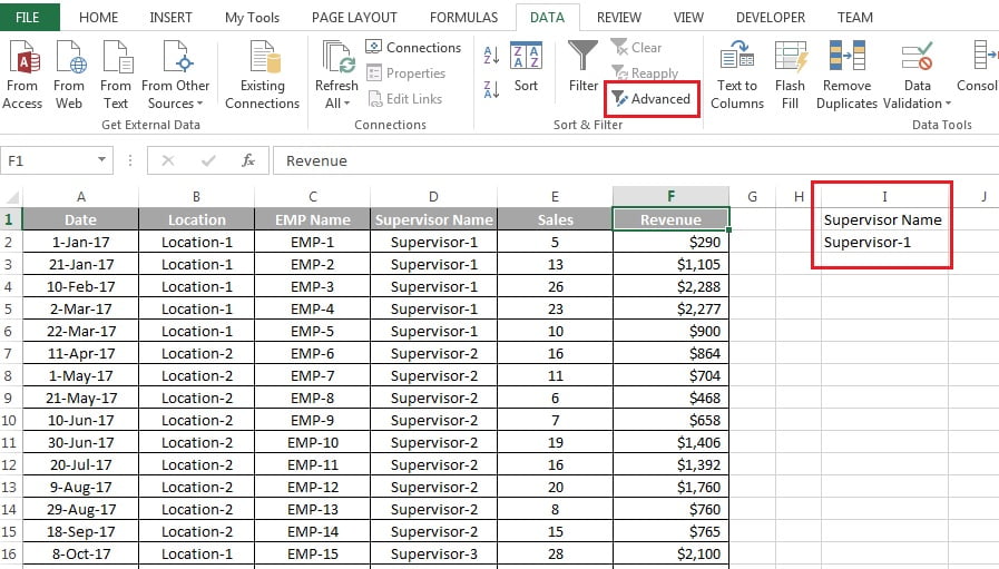
The example list holds sales records with a Supervisor column, and the goal is to show only Supervisor-1. The criteria range is H1:H2: the header Supervisor in H1 and the value Supervisor-1 in H2.

1. Type the header exactly as it appears in the data, then the criterion in the cell beneath it.
2. Click any cell in the list and choose Data > Sort & Filter > Advanced.

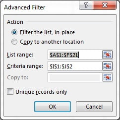
3. In the Advanced Filter dialog keep Filter the list, in-place. Excel fills List range with the current region; check that it includes the header row.
4. Click in Criteria range and select H1:H2, the header and the criterion together.
5. Click OK.

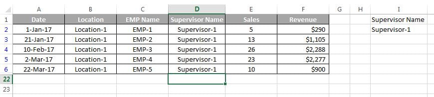
Only the Supervisor-1 rows remain and the hidden row numbers turn blue, exactly as with AutoFilter. To show everything again click Data > Sort & Filter > Clear.

How to filter by multiple fields with AND and OR

To show Supervisor-1 rows where Sales is greater than 10, add a second header Sales beside Supervisor and type >10 beneath it on the same row as Supervisor-1. Two conditions on one row mean AND.

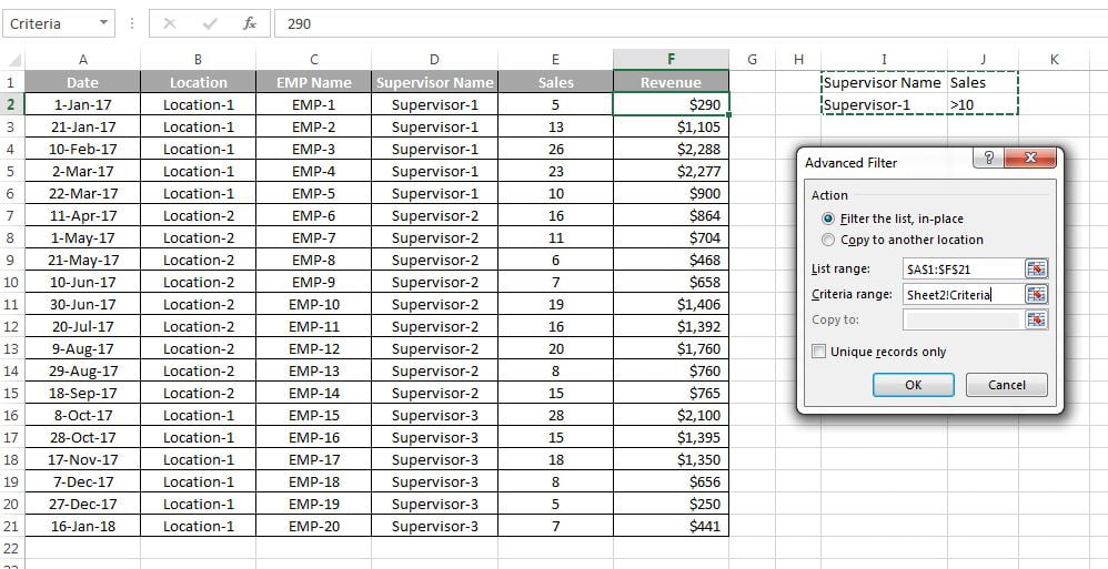
Run Data > Advanced again and extend Criteria range to H1:I2. Only Supervisor-1 rows with more than 10 sales survive. For Supervisor-1 or Sales above 10, move >10 down to row 3 under the Sales header, leave H3 blank, and select H1:I3 as the criteria range. Excel now returns any row that satisfies either row of conditions.

How to copy the results to another location

Filtering in place hides rows. Copying writes the matching rows to a new range, which is what you want for a report extract or a mailing list.

1. Select a cell on the sheet where the results should go. If the destination is a different worksheet, start from that sheet, because the Copy to range must be on the active sheet.
2. Choose Data > Sort & Filter > Advanced and select Copy to another location.
3. Set List range to the data, including headers, on whichever sheet it lives.
4. Set Criteria range to your criteria block.
5. Click in Copy to, select one empty cell, and click OK. Excel writes the headers and the matching rows starting at that cell.

To copy only some columns, type the headers you want, in any order, in the destination row before you open the dialog, then select those header cells as the Copy to range. Excel fills only those columns. This is the quickest way to reorder or trim a report without formulas.

How to extract unique records

The Unique records only box removes duplicate rows from the output. Combine it with Copy to another location to build a distinct list.

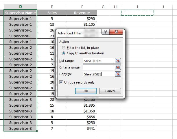
1. Select the column you want to de-duplicate, including its header, for example the Supervisor column.
2. Choose Data > Sort & Filter > Advanced and select Copy to another location.
3. Leave Criteria range empty, click in Copy to and select a single empty cell where the list should start.
4. Tick Unique records only and click OK.

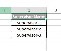
A de-duplicated list of supervisors appears at the Copy to cell. Select two or more columns in the list range and you get unique combinations instead, for example every Location and Supervisor pair that appears in the data.

How to use a formula as the criteria

Formula criteria let you filter on anything you can calculate: above-average values, weekends, rows where two columns disagree, or the top 10 by rank. The rules differ from normal criteria:

• The header cell above the formula must be blank or a label that does not match any list header, such as “Above average”.
• The formula must return TRUE or FALSE and must refer to the first data row with a relative reference, for example D2. Excel tests it against every row in turn.
• Any range the formula compares against must use absolute references, such as $D$2:$D$100.

Example: with Sales in column D, the criteria formula =D2>AVERAGE($D$2:$D$100) keeps only above-average rows. Ignore the TRUE or FALSE the cell itself shows; it only reflects row 2. You can place a formula criterion on the same row as ordinary criteria to combine them with AND.

Worked example

The list below sits in A1:D7. The criteria are in F1:H3.

Row	Location	Supervisor	Sales
2	Delhi	Supervisor-1	12
3	Mumbai	Supervisor-2	8
4	Delhi	Supervisor-1	6
5	Pune	Supervisor-3	15
6	Mumbai	Supervisor-1	11
7	Delhi	Supervisor-2	9

Goal: Supervisor-1 rows with Sales above 10, plus every row from Pune regardless of supervisor. Criteria range F1:H3:

Location	Supervisor	Sales
	Supervisor-1	>10
Pune

1. Click cell A1 and open Data > Advanced.
2. List range $A$1:$D$7, Criteria range $F$1:$H$3, Filter the list in-place, OK.

Result: rows 2, 5 and 6. Row 2 and row 6 pass the first criteria row (Supervisor-1 AND Sales above 10); row 5 passes the second (Pune). Row 4 fails because 6 is not above 10. Swap the criteria for a blank header with =D2>AVERAGE($D$2:$D$7) and the average of 10.17 returns the same three rows: 12, 15 and 11.

Limitations and the Excel 365 alternative

Advanced Filter is a one-time action. If the data or the criteria change, nothing updates until you run it again, and the copied output is plain values with no link to the source. The Copy to range must be on the active sheet and the criteria headers must match precisely.

In Excel 365 and Excel 2021 the FILTER and UNIQUE functions do the same jobs as live formulas that recalculate automatically. Multiply conditions for AND and add them for OR:

=FILTER(A2:D7,(C2:C7="Supervisor-1")*(D2:D7>10),"No match")
=FILTER(A2:D7,(C2:C7="Supervisor-1")+(D2:D7>10))
=UNIQUE(C2:C7)
=SORT(UNIQUE(B2:C7))

Use Advanced Filter when you need a static extract, when the workbook must open in Excel 2019 or earlier, or when you are recording a macro. Use FILTER and UNIQUE when the result should stay current. The dynamic functions are covered in the SORT, SORTBY, FILTER and UNIQUE lesson.

Tips and common mistakes

• Copy the headers, do not retype them. A trailing space or different capitalisation in a criteria header silently returns nothing. Copy and paste from the list.
• Never include a blank row in the criteria range. An empty row matches every record, so the filter appears to do nothing.
• Force exact text matches. Plain text matches the start of the cell. Enter ="=Delhi" to match only Delhi. Excel displays it as =Delhi.
• Numbers stored as text ignore comparisons. If >5000 returns nothing, convert the column with Text to Columns or multiply by 1 first.
• Record a macro. Advanced Filter records cleanly, so a monthly extract becomes one button. Set the Copy to cell first so the recorded code writes to the right place.

Errors and how to fix them

Message or symptom	Cause	Fix
The extract range has a missing or invalid field name	A header typed in the Copy to range does not match a list header, or the Copy to range includes an empty header cell	Copy the headers from the list; select only the cells that contain headers, or a single empty cell
You can only copy filtered data to the active sheet	You started from the source sheet and pointed Copy to at another sheet	Cancel, activate the destination sheet, open Advanced Filter from there and set the List range back to the source
No rows returned	Criteria header does not match, or numbers are stored as text	Recopy the header; convert the column to numbers
Every row returned	A blank row inside the criteria range	Reselect the criteria range so it ends at the last filled row
Formula criterion filters nothing or everything	The header above the formula matches a list header, or the formula uses an absolute reference to the test cell	Clear the header; reference the first data row relatively, such as D2
Results are out of date	Advanced Filter does not recalculate	Rerun it, or switch to FILTER in Excel 365

Practice exercise

Download the Sort and Filter practice file and complete these tasks on the sales sheet.

1. Build a criteria range that returns Supervisor-1 rows with Sales above 10, then edit it so it returns Supervisor-1 rows or any row with Sales above 10. Compare the counts.
2. Add a third criteria row so any Supervisor-3 row is included as well, and filter in place.
3. From a new sheet, copy every row that is not from Delhi (<>Delhi) to that sheet, but only the Supervisor and Sales columns.
4. Extract a unique list of Location and Supervisor combinations with Unique records only.
5. Use a blank-header formula criterion to show rows where Sales is above the column average, then rebuild the same result with the FILTER function if you have Excel 365.

Key takeaways

• Advanced Filter lives at Data > Sort & Filter > Advanced and reads its conditions from a criteria range on the worksheet.
• Conditions on the same row are AND; conditions on separate rows are OR; a blank row matches everything.
• Comparison operators, wildcards and ="=text" control how text and numbers are matched.
• A formula under a blank header filters on any calculated condition; reference the first data row relatively.
• Copy to another location must target the active sheet; type headers in the destination to copy selected columns.
• Unique records only extracts a distinct list; FILTER and UNIQUE are the live alternatives in Excel 365.

Related lessons

• Excel Sort and Filter course hub
• Text, Number and Date Filters in AutoFilter
• Remove Duplicates and Highlight Duplicates in Excel
• SORT, SORTBY, FILTER and UNIQUE functions
• FILTER function with examples and UNIQUE and the other dynamic array functions
• Microsoft Support: Filter by using advanced criteria

Frequently asked questions

Where is Advanced Filter in Excel?

Advanced Filter is on the Data tab in the Sort & Filter group, labelled Advanced, next to the Filter and Clear buttons. Click any cell inside your list first so Excel proposes the List range for you. The keyboard route is Alt, A, Q. It is available in Excel 365, 2021, 2019 and 2016 for Windows and Mac, but not in Excel for the web.

How do I use OR conditions in Advanced Filter?

Put each alternative on its own row under the headers and include every row when you select the criteria range. Conditions on the same row are combined with AND, conditions on different rows with OR. For Supervisor-1 or Sales above 10, place Supervisor-1 in row 2 under Supervisor and >10 in row 3 under Sales, leaving the other cells blank.

Why does Advanced Filter return no rows or every row?

No rows usually means a criteria header does not match the list header exactly, often because of a trailing space, or the numbers are stored as text so >10 finds nothing. Every row means the criteria range includes a blank row, which matches all records. Reselect the range so it covers only the header and the filled criteria cells.

Can Advanced Filter copy results to another worksheet?

Yes, but you must start from the destination sheet. Select a cell there, open Data > Advanced, choose Copy to another location, set List range to the data on the source sheet, set the Criteria range, and pick a Copy to cell on the current sheet. Starting from the source sheet gives the error that you can only copy filtered data to the active sheet.

Is Advanced Filter the same as the FILTER function?

They solve the same problem differently. Advanced Filter is a dialog that produces a static result and works in every version of Excel. FILTER is a dynamic array function in Excel 365 and 2021 that recalculates whenever the data or criteria change and spills its result automatically. Use FILTER for live reports and Advanced Filter for one-off extracts, older workbooks and recorded macros.

Want the finished version? Ready-made Excel dashboards, trackers and VBA systems are available at NextGenTemplates.com.