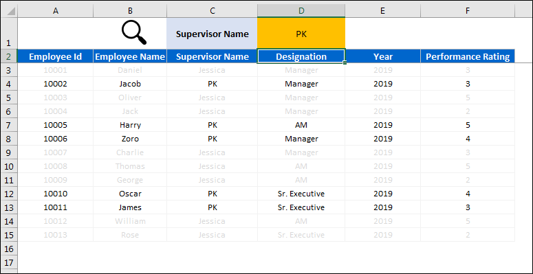
Search Text from Specific or All Columns in Excel (No VBA)

Want to search text from specific or all columns in Excel and see the matching rows instantly, without filters or VBA? In this tutorial you will build a small search box with conditional formatting. Type a name, an ID or even two letters, and every row that does not match fades to light grey, so the matches stand out. You will build two versions on an employee performance list: one that searches only the column you pick from a drop-down, and one that searches every column at once. Along the way you will see exactly how SEARCH, ISERROR, MATCH, ADDRESS and INDIRECT work together.

Search text from specific or all columns in Excel: Supervisor Name selected, PK typed in the search box and non-matching rows greyed out — Search in a specific column: Supervisor Name is selected and PK is typed, so only PK’s employees stay dark.

⬇️ Download the Practice File
Specific-column and all-columns search sheets · .xlsx (no macros) · Excel 2010 and later

Table of Contents

Watch the Video Tutorial

PK demonstrates both searches, then builds the rules step by step: first testing each formula in a helper column, then moving it into conditional formatting.

What You Will Build

A search box (cell D1) where you type full or partial text.
A column picker (cell C1), a drop-down of the table headers.
A specific-column search that checks only the selected column.
An all-columns search that checks the whole row.
Row-level highlighting: non-matching rows fade to light grey and matching rows keep their normal look.

Example Data to Search Text from Specific or All Columns in Excel

Both sheets in the practice file use the same employee performance list in A2:F15: Employee Id, Employee Name, Supervisor Name, Designation, Year and Performance Rating, with 13 employees from 10001 Daniel to 10013 Rose. Supervisors are Jessica and PK, and designations are Manager, AM and Sr. Executive. Row 1 holds the search controls, and the rules are applied to the data range A3:F15.

As PK notes in the original post, this trick is best for small data sets. The formulas run for every cell in the range, so on many thousands of rows a filter is faster.

Part 1: Search Text from a Specific Column

Step 1: Set up the search controls

Type your search text in D1 and give it a yellow fill so users know where to type. PK adds a magnifier icon in B1 for a search-bar look.
Select C1, go to Data → Data Validation, choose List and set the source to =$A$2:$F$2. C1 now offers every column header.
Pick Employee Name in C1 to start.

Step 2: Test the logic in a helper column

Conditional formatting needs a formula that returns TRUE or FALSE. PK tests it on the sheet first, which is a good habit. Next to row 3, enter:

=SEARCH($D$1,B3)

SEARCH returns the position of the text when it is found (for example 1) and a #VALUE! error when it is not. Wrap it in ISERROR to turn that into a clean TRUE or FALSE:

=ISERROR(SEARCH($D$1,B3))

Fill it down. Rows where the name does not contain the search text return TRUE. Type Ja in D1 and you get FALSE for Jacob, Jack and James, because SEARCH finds a partial match and ignores upper and lower case.

Step 3: Make the column dynamic

The test formula only looks at column B. To follow whatever header is picked in C1, you need the right cell address for each row.

First get the column number of the selected header:

=MATCH($C$1,$A$2:$F$2,0)

With Supervisor Name selected this returns 3. Then build the cell address for the current row:

=ADDRESS(ROW(A3),MATCH($C$1,$A$2:$F$2,0),3)

This returns the text $C3. The third argument, 3, means absolute column and relative row. Switch C1 to Employee Name and it returns $B3 instead. Because ADDRESS returns text, wrap it in INDIRECT to turn it into a real reference, and put everything inside the ISERROR and SEARCH test.

Step 4: Add the conditional formatting rule

Select the data without headers, A3:F15, with A3 as the active cell.
Go to Home → Conditional Formatting → New Rule and choose Use a formula to determine which cells to format.
Enter the formula from the practice file:

=ISERROR(SEARCH($D$1,INDIRECT(ADDRESS(ROW(A3),MATCH($C$1,$A$2:$F$2,0),3))))

Edit Formatting Rule window with Use a formula to determine which cells to format and the ISERROR SEARCH INDIRECT ADDRESS formula — The formatting rule window with the specific-column formula, shown here from Edit Rule.

Click Format, open the Font tab and choose a light grey colour. The practice file uses White, Background 1, Darker 15%, plus very light cell borders.
Click OK twice.

Format Cells window on the Font tab with a light grey font colour selected — Pick a light grey font so non-matching rows fade into the background.

To edit the rule later, press Alt, O, D (or Home → Conditional Formatting → Manage Rules), select the rule and click Edit Rule. You can now delete the helper column.

How the formula works

MATCH($C$1,$A$2:$F$2,0) finds the position of the chosen header, for example 3 for Supervisor Name.
ROW(A3) gives the row number. A3 is relative, so on row 7 it becomes A7 and returns 7.
ADDRESS(row, column, 3) joins them into text such as $C7.
INDIRECT(...) turns that text into a live reference to cell C7.
SEARCH($D$1, ...) looks for the search text inside that cell and errors if it is missing.
ISERROR(...) returns TRUE for rows with no match, and only those rows get the grey font.

Because the address always points at the selected column for that row, every cell in the row (A to F) gets the same answer, so the whole row fades together.

Part 2: Search Text in All Columns

For the second sheet you do not need the column picker. Instead of reading one cell, join the whole row into one string and search that. The rule is the same apart from the formula:

=ISERROR(SEARCH($D$1,CONCATENATE($A3,$B3,$C3,$D3,$E3,$F3)))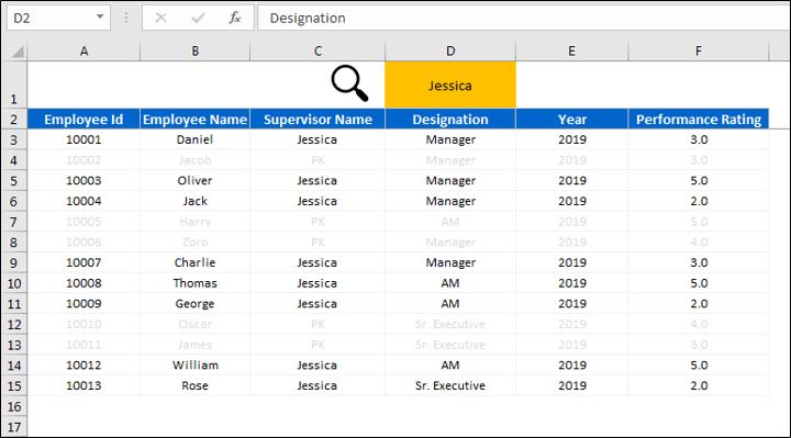

Search in all columns in Excel: Jessica typed in the search box and rows without Jessica greyed out — Search in all columns: every row containing Jessica in any column stays dark.

CONCATENATE turns row 3 into one string, 10001DanielJessicaManager20193, so the search text can be found anywhere in the row. Type PK, Manager or Jack in D1 and the matching rows stay dark.

The dollar sign that makes it work

In the video the first attempt did not fade the whole row. The fix is the $ before each column letter: $A3 to $F3. When the rule is evaluated for cell D7, the references still point to columns A to F of row 7. Without the dollar signs, each cell would shift its own range to the right and the result would differ across the row. The same applies in Part 1 if you build the simple version with $B3.

A Lighter Version of the Formulas

Addition, not from the video: INDIRECT is a volatile function, so Excel recalculates it after every change in the workbook. On a bigger list you can get the same specific-column result without it:

=ISERROR(SEARCH($D$1,INDEX($A3:$F3,MATCH($C$1,$A$2:$F$2,0))))

INDEX picks the cell from the current row at the matched position, so there is no text address to convert. For the all-columns search in Excel 2019 or Microsoft 365, TEXTJOIN with a separator stops matches that run across two cells:

=ISERROR(SEARCH($D$1,TEXTJOIN("|",TRUE,$A3:$F3)))

Modern Excel Alternative: FILTER

Addition, not from the video: in Microsoft 365 you can also return the matching rows to a separate area instead of greying out the rest:

=FILTER(A3:F15,ISNUMBER(SEARCH(D1,INDEX(A3:F15,0,MATCH(C1,A2:F2,0)))),"No match")

Use the conditional formatting method when you want to keep the full list in view, and FILTER when you only want the results.

Common Errors and Fixes

Only some cells in a row fade

The column references are missing the $ sign. Use $A3 to $F3 (or $B3 in the simple version) so every cell in the row checks the same cells.

The highlighting is shifted by one row

The active cell was not A3 when you created the rule. Select A3:F15 starting from A3, or edit the rule so the row reference matches the first row of the selection.

Every row stays dark when the search box is empty

That is expected: SEARCH treats empty search text as found at position 1, so nothing is greyed out until you type something.

Every row fades as soon as you pick a column

The header in C1 must match the header row exactly. If it does not, MATCH returns #N/A, ISERROR turns that into TRUE and every row goes grey. Keep the drop-down source as $A$2:$F$2 so a typo cannot get in.

Tips

SEARCH ignores case. If you need case-sensitive matching, use FIND in the same position.
Partial text works, so two or three letters are often enough to narrow the list.
Grey text works better than a bright fill here: matches stay readable and the sheet stays calm.
Test every conditional formatting formula in a helper column first, exactly as PK does, then copy it into the rule.
Microsoft explains formula-based rules in its guide to using conditional formatting to highlight information.

Want It Ready-Made?

For ready-built highlighting, the Dynamic Conditional Formatting in Excel template on NextGenTemplates.com gives you rule-driven highlighting to reuse, and the Employee Performance Tracking Report in Excel suits data like the list in this tutorial. Browse more Excel templates there. To master SEARCH, MATCH, INDEX and the other formulas used here, see the course Excel + AI Mastery: 100 Essential Formulas and Real-World Projects.

Frequently Asked Questions

How do I highlight rows that contain specific text in Excel?

Select the data, add a conditional formatting rule with a formula, and use SEARCH to look for the text in each row. This tutorial greys out rows without a match so the matching rows stand out.

Is the search case-sensitive?

No. SEARCH ignores upper and lower case and allows partial matches. Use FIND instead if you need a case-sensitive search.

Can I search in more than one column at a time?

Yes. The all-columns version joins the whole row with CONCATENATE and searches that combined text, so a match in any column keeps the row visible.

Why does the formula use INDIRECT and ADDRESS?

ADDRESS builds the cell address of the selected column for each row as text, and INDIRECT turns that text into a real reference that SEARCH can read.

Does this work on large data sets?

It is designed for small lists. INDIRECT recalculates often, so on large tables use the INDEX version shown above or a filter.

About the Author

PK is a Microsoft Excel expert and trainer and the founder of PK: An Excel Expert and NextGenTemplates.com. He has been teaching Excel, VBA, Power Query and Power BI since 2016 on his YouTube channel.

Conclusion

With one conditional formatting rule you can search text from specific or all columns in Excel and see the matching rows at a glance. A drop-down in C1, a search box in D1, and a SEARCH test wrapped in ISERROR are all it takes, with MATCH, ADDRESS and INDIRECT pointing at the chosen column, or CONCATENATE covering the whole row. Download the practice file, try a few searches, and then add the same search box to your own lists.