In this article you will learn how to show Change% in a pivot table. For example, you have month wise sales and revenue in your pivot and you have to show the change% in sales and revenue in compare of previous month.
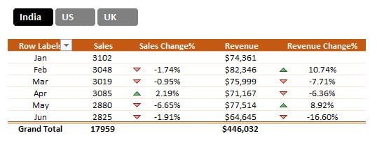
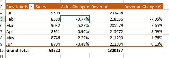
We will show the change% as given in below image.
Change% in Pivot Table
Steps show the change% in a pivot table-
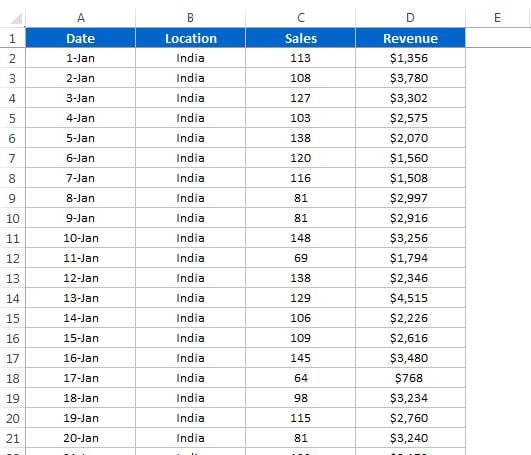
- Lets say we have below given sales data.
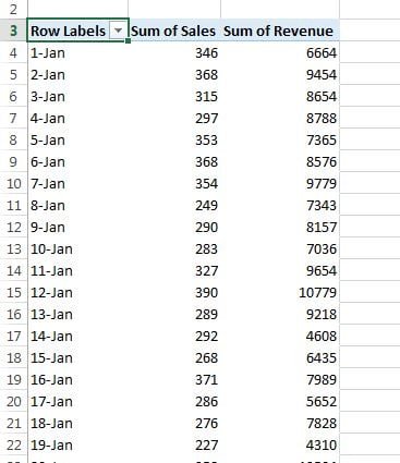
- Create a pivot table for above data.
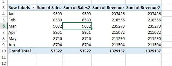
- Drag the Date in Rows.
- Sales and Revenue in Values.
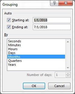
- After grouping, drag the Sales and Revenue again in Values.
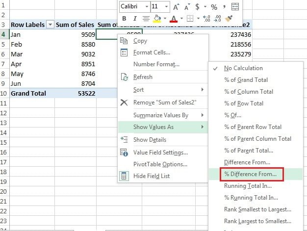
- Right click on in the Sum of Sales2.
- Go to the Show Value As >>%Difference From…
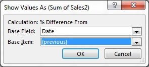
- Select the Base Field as Date.
- Select the Base Item as (previous).
- Repeat the same activity for Sum of Revenue2 column.
- Change the column name Sum of Sales2 as Sales Change%.
- Change the column name Sum of Revenue2 as Revenue Change%.
- Change the pivot style.
- Click anywhere on Sales Change % column.
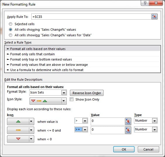
- Go to Home table>>Conditional Formatting>>New Rule
- Select All Cells showing “Sales Change%” value
- Select Format All Cells based on there values in Rule Type.
- Choose Format Style as Icon Set.
- Select the option as given in below image-
- Repeat the same activity with the Revenue Change%.
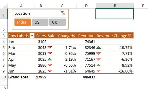
- Insert a Slicer for Location and change the Slicer style.
Click here to download the this excel workbook.
Watch the step by step tutorial:
Visit our YouTube channel to learn step-by-step video tutorials