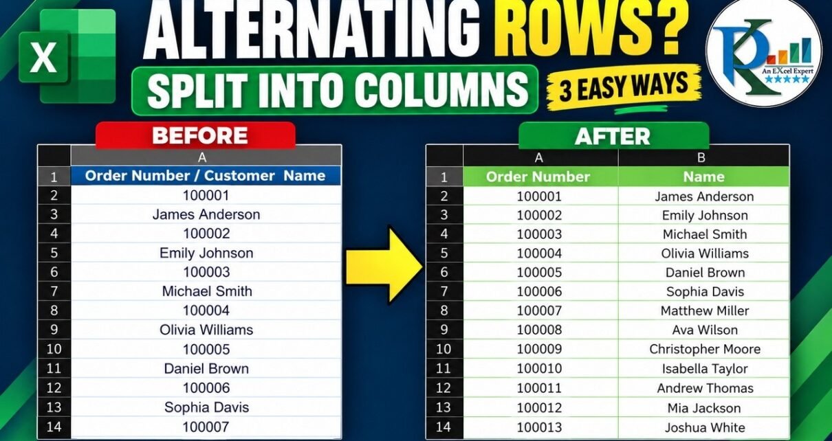
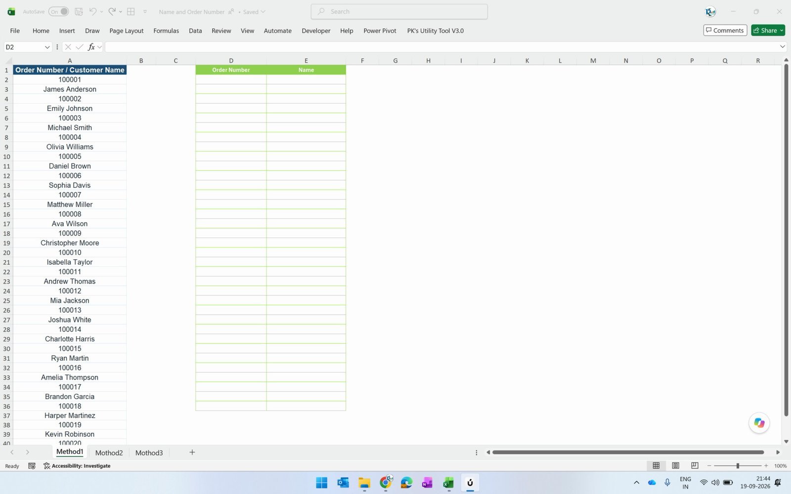
You open a file and the whole list has been pasted into one single column: an order number, then a customer name, then another order number, then another name — all the way down. In our sample that is 40 rows in column A (A2:A41): 20 order numbers (100001 to 100020) and 20 customer names, stacked alternately.
Copying them into two clean columns by hand works, but with a thousand rows it is an afternoon gone. In this tutorial you will learn 3 tricks to separate the number and text from an Excel column — one click-based method and two formulas — and, more importantly, which one to trust when your data is not perfectly patterned.
Free ZIP — practice workbook + finished solution workbook (no sign-up needed)
Watch the Video Tutorial
Video overview. The 5-minute walkthrough starts with the raw list — order numbers and customer names alternating in column A — and shows why copy-and-paste is the wrong tool for the job. Trick 1 uses Go To Special: select the column, press Ctrl + G, click Special…, choose Constants, leave only Numbers ticked, then copy and paste as values into the Order Number column, and repeat with Text for the names. Trick 2 replaces all of that with one formula, =WRAPROWS(A2:A41,2), which folds the single column into two — and the video shows exactly what goes wrong when you select extra rows. Trick 3 is the one worth remembering: FILTER combined with ISNUMBER and ISTEXT. It reads the data type of every cell instead of counting positions, so it keeps working even when someone adds an extra name and breaks the pattern.
What You Will Build
- A clean Order Number column (D) containing only the 20 numeric values.
- A clean Name column (E) containing only the 20 customer names.
- Three working versions of the same result — one manual, two formula-driven — on three separate sheets so you can compare them side by side.
- A dynamic version that survives a broken pattern.
The Sample Data
Every sheet in the practice file holds the same source list in column A:
| Cell | Value | Data type |
|---|---|---|
| A1 | Order Number / Customer Name | Header |
| A2 | 100001 | Number |
| A3 | James Anderson | Text |
| A4 | 100002 | Number |
| A5 | Emily Johnson | Text |
| … | … | … |
| A40 | 100020 | Number |
| A41 | Evelyn Clark | Text |
The destination columns are D — Order Number and E — Name. That single fact — numbers are numbers and names are text — is what all three tricks exploit.
Trick 1: Go To Special (the no-formula method)
Excel can select every numeric cell or every text cell in a range for you. Once they are selected, a single copy-and-paste moves them out.
Step 1 — Select the column
Click the column A header (or select A2:A41) so the whole mixed list is highlighted.
Step 2 — Press Ctrl + G and click Special…
The Go To window opens. Click the Special… button in the bottom-left corner, or press Alt + S.

Step 3 — Choose Constants, keep only Numbers
In the Go To Special window, click the Constants radio button. Four checkboxes light up underneath it — Numbers, Text, Logicals and Errors. Untick everything except Numbers and click OK.
Careful: pressing the N key here does not jump to Constants — it selects Notes. Click the Constants option with the mouse.

Step 4 — Copy the selection
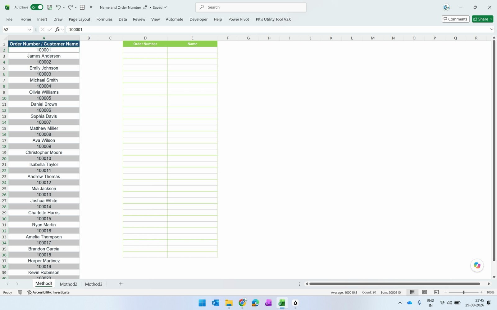
Excel now has only the 20 numeric cells selected — the customer names are skipped entirely. Press Ctrl + C.
Step 5 — Paste as values into the Order Number column
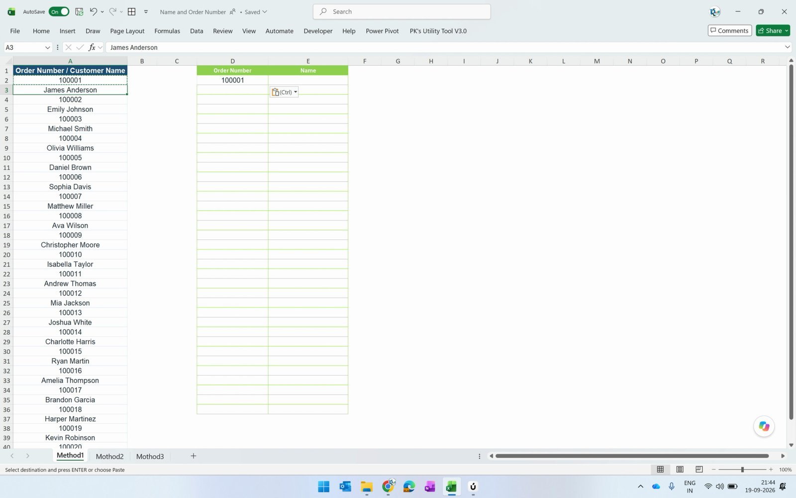
Click cell D2 and paste as values. The 20 order numbers land in a continuous block with no gaps.
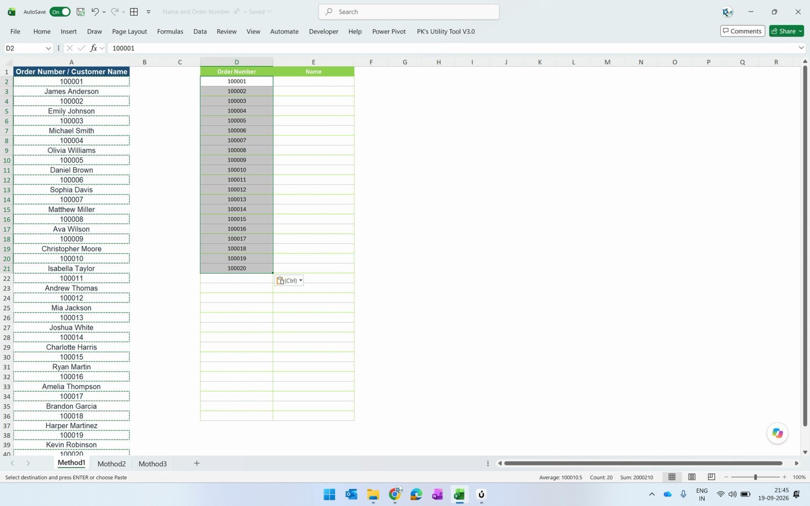
Step 6 — Repeat with Text for the names
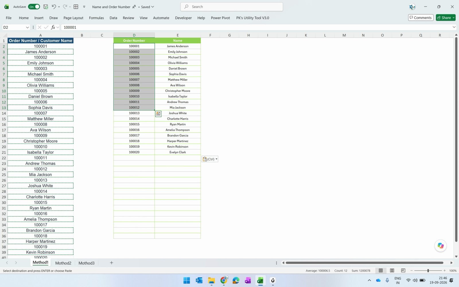
Select column A again, press Ctrl + G → Special… → Constants, and this time keep only Text ticked. Click OK, copy, then paste as values into E2.

Both columns are now filled, and it took the same number of clicks whether the list had 40 rows or 4,000.
Trick 2: The WRAPROWS Formula
WRAPROWS takes a one-dimensional list and wraps it into rows of a fixed width. Our list repeats in pairs — number, name, number, name — so a wrap count of 2 rebuilds the two columns in a single step.
In cell D2, type:
=WRAPROWS(A2:A41,2)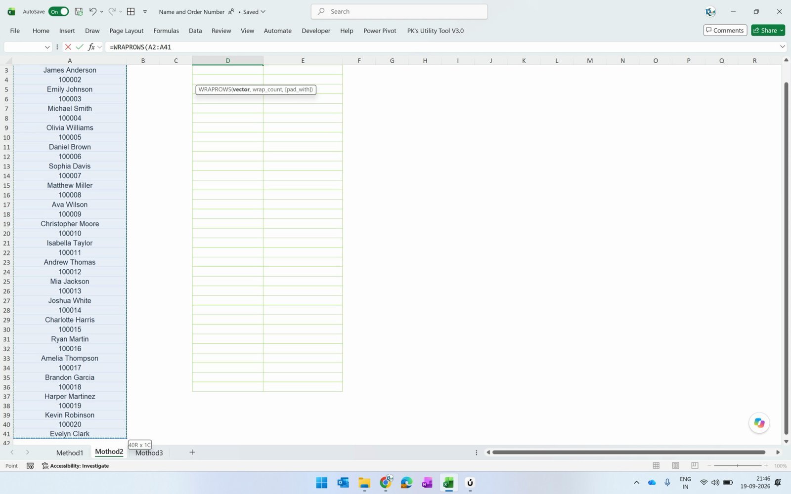
The second argument is the wrap count. We have exactly two kinds of value per repetition — an order number and a customer name — so the wrap count is 2. Press Enter and the whole grid spills out at once.
Watch out for extra rows
If you select more rows than the list actually uses (or select the entire column), the empty cells come through as zeros.
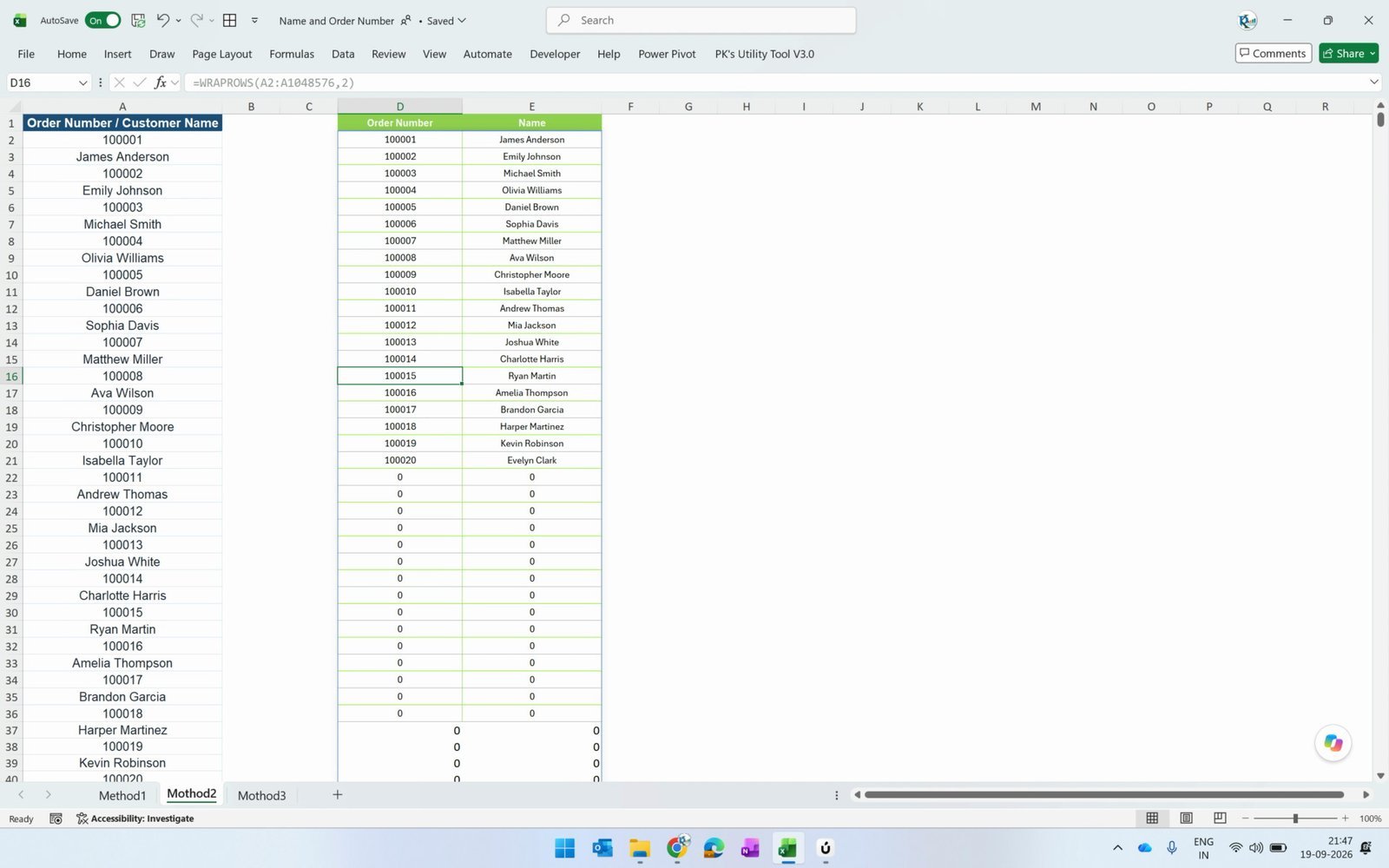
Either filter the zeros out afterwards, or simply tighten the range to the last used row — A41 in our file:
=WRAPROWS(A2:A41,2)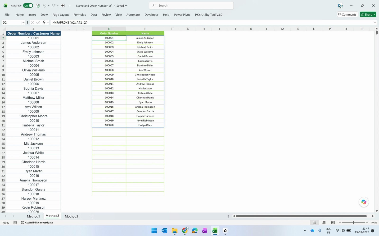
The catch: WRAPROWS counts positions, not data types. It assumes the pattern never breaks. Put one extra customer name at row 4 and every value below it shifts by one — names start landing in the Order Number column. If your data comes from someone else, this is a real risk.
Trick 3: FILTER with ISNUMBER and ISTEXT (the dynamic one)
This is the method worth memorising. Instead of counting positions, FILTER asks Excel a question about every cell: is this a number? or is this text? — and keeps only the ones that answer yes.
The order numbers
In cell D2:
=FILTER(A2:A41,ISNUMBER(A2:A41))FILTER takes the array first, then the include argument. ISNUMBER(A2:A41) returns TRUE for every numeric cell and FALSE for every name, so only the order numbers survive.

The customer names
In cell E2, the formula is identical except for one function — swap ISNUMBER for ISTEXT:
=FILTER(A2:A41,ISTEXT(A2:A41))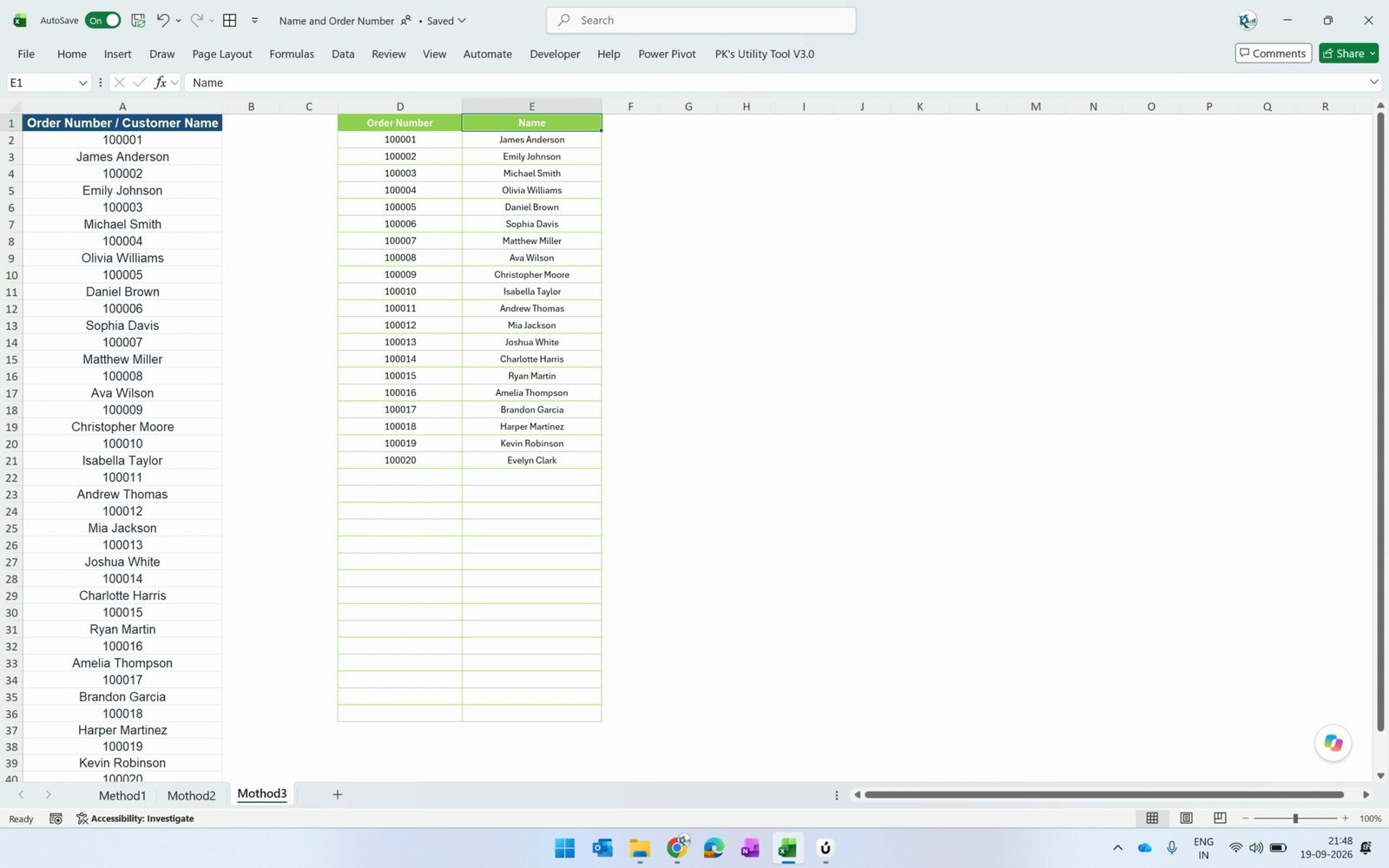
Why this one survives a broken pattern
Add an extra customer name anywhere in column A and run the test. WRAPROWS would shift everything below it — but FILTER simply picks up one more name in the Name column and leaves the Order Number column completely untouched.
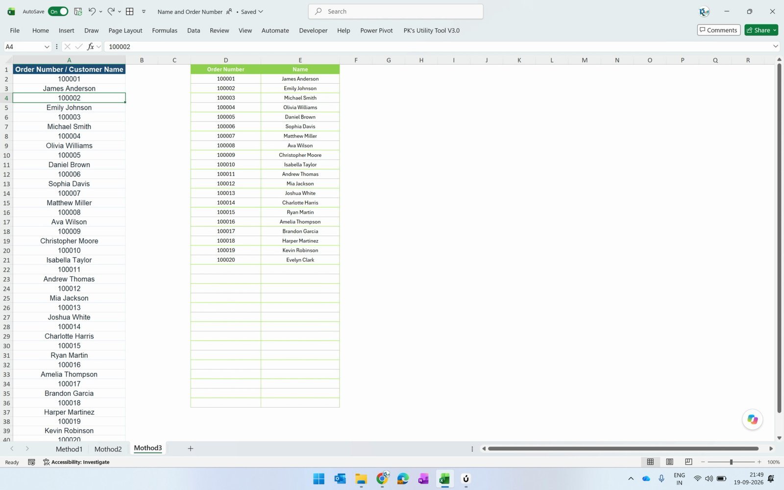
Both formulas also update themselves the moment the source list changes — no re-running, no re-pasting.
Which Method Should You Use?
| Trick 1 — Go To Special | Trick 2 — WRAPROWS | Trick 3 — FILTER + ISNUMBER / ISTEXT | |
|---|---|---|---|
| Type | Manual (clicks) | Formula | Formula |
| Result updates automatically | No — values only | Yes | Yes |
| Needs a strict pattern | No | Yes | No |
| Handles an extra name | Yes | No — everything shifts | Yes |
| Excel version | All versions | Microsoft 365 / Excel 2021+ | Microsoft 365 / Excel 2021+ |
| Best for | A one-off clean-up in an old version | A perfectly alternating list | Data you did not create yourself |
Tips Worth Remembering
- Numbers stored as text will be ignored by ISNUMBER. If an order number is left-aligned in the cell, Excel is treating it as text. Convert it first (Data → Text to Columns → Finish is the quickest fix).
- Always paste as values in Trick 1. A normal paste brings the source formatting with it and can overwrite your column styling.
- Keep the range tight. Both
WRAPROWSandFILTERbehave better onA2:A41than on the whole of column A. - Use a Table if the list keeps growing — a structured reference expands on its own, so the formulas never need editing.
ISTEXTis the mirror ofISNUMBER, so the twoFILTERformulas always split the list cleanly with nothing left behind.
Frequently Asked Questions
Which Excel versions support WRAPROWS and FILTER?
FILTER arrived with dynamic arrays in Microsoft 365 and Excel 2021. WRAPROWS is newer and is available in Microsoft 365 and Excel 2021 onward. If you are on Excel 2019 or older, use Trick 1 (Go To Special) — it works in every version.
Why does WRAPROWS return zeros?
Because the range you selected includes empty cells below the last row of data. WRAPROWS treats a blank cell as a zero. Shorten the range to the last used row, or wrap the formula in a filter to drop the zeros.
What is the wrap count in WRAPROWS?
It is how many values go into each row before the function wraps to the next one. Our list repeats in pairs — one order number and one customer name — so the wrap count is 2.
My order numbers are not being picked up by ISNUMBER. Why?
They are almost certainly stored as text. A quick check: numbers align right in a cell by default, text aligns left. Convert the column to real numbers and the formula will start returning them.
Can I do this without any formula at all?
Yes — that is Trick 1. Ctrl + G → Special… → Constants → Numbers only, copy, paste as values; then repeat with Text. The result is static values rather than a live formula.
Does pressing N select Constants in the Go To Special window?
No. N selects Notes, which is a different option entirely. Click Constants with the mouse — this is a mistake that is very easy to make.
What happens if the pattern in my column is broken?
Use Trick 3. FILTER with ISNUMBER and ISTEXT reads the data type of each cell rather than its position, so an extra name (or an extra number) never shifts the other column.
Download the Practice File
The free ZIP contains two workbooks — a practice file with the raw mixed column and empty result columns, and a solution file with all three tricks already built so you can compare your work.
Separate-Number-Text-Practice-Files.zip — practice + solution workbook
Related Tutorials
- FILTER and ISTEXT Function in Excel with Examples
- WRAPROWS Function in Excel with Examples
- WRAPCOLS Function in Excel with Examples
Microsoft’s own reference for the function used in Trick 3 is here: FILTER function — Microsoft Support.
About the Author
I am PK, an Excel and data-visualisation trainer, and the author of PK: An Excel Expert. I publish free Excel, Power Query, Power Pivot and Power BI tutorials with a downloadable practice file for every single one.
Conclusion
All three tricks give you the same two clean columns from one messy one. Go To Special is the version that works in every copy of Excel ever shipped. WRAPROWS is the shortest formula — as long as your list alternates perfectly. And FILTER with ISNUMBER and ISTEXT is the one I would actually put into a working file, because it asks each cell what it is rather than trusting where it sits.
Download the practice file, try all three on the same data, then break the pattern on purpose and watch which one keeps its nerve.