VBA: Filter Data with Multiple Values

In this article you will learn how we can use an excel range as a filter criteria and paste the filtered data on another worksheet.

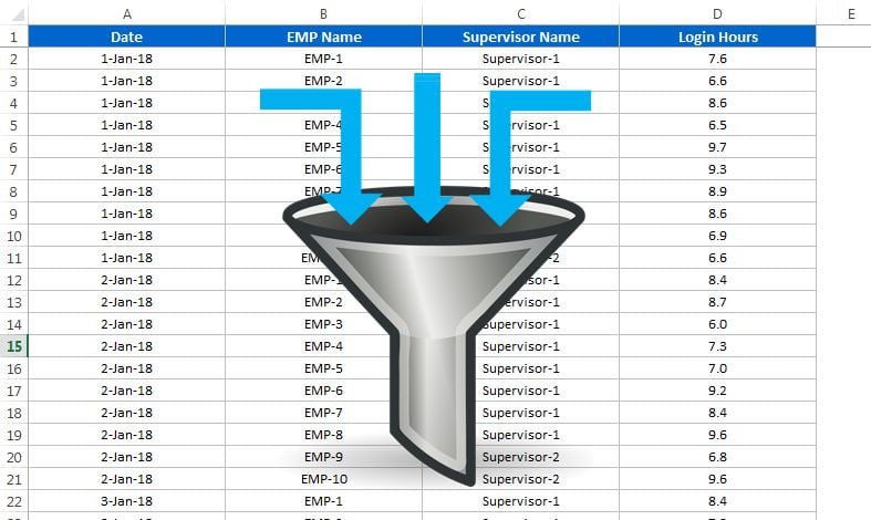
For example, we have below data in “Data” worksheet.

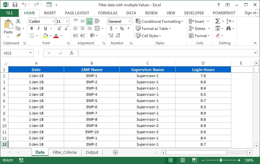
We have below given Employee list whose data has to be filtered and copied on “Output” worksheet.

Here we have created a macro to get the desired output.

Below is the VBA code:

• Copy the below given code and go to Visual Basic Editor (Press Alt+F11)
• Insert a module (Press  Alt+I+M)
• Paste this code in the module.
• Save as the workbook as Macro enable workbook.
• Insert a rectangle shape in “Filter_Criteria” worksheet and right click on this shape and assign “Filter_My_Data()” macro.

Option Explicit

Sub Filter_My_Data()

Dim Data_sh As Worksheet

Dim Filter_Criteria_Sh As Worksheet

Dim Output_sh As Worksheet

Set Data_sh = ThisWorkbook.Sheets("Data")

Set Filter_Criteria_Sh = ThisWorkbook.Sheets("Filter_Criteria")

Set Output_sh = ThisWorkbook.Sheets("Output")

Output_sh.UsedRange.Clear

Data_sh.AutoFilterMode = False

Dim Emp_list() As String

Dim n As Integer

n = Application.WorksheetFunction.CountA(Filter_Criteria_Sh.Range("A:A")) - 2

ReDim Emp_list(n) As String

Dim i As Integer

For i = 0 To n

    Emp_list(i) = Filter_Criteria_Sh.Range("A" & i + 2)

Next i

Data_sh.UsedRange.AutoFilter 2, Emp_list(), xlFilterValues

Data_sh.UsedRange.Copy Output_sh.Range("A1")

Data_sh.AutoFilterMode = False

MsgBox ("Data has been Copied")

End Sub

Click here to download Excel template.

Watch the step by step video tutorial: