Dynamic Project Planner Gantt Chart in Excel (Daily/Weekly View)

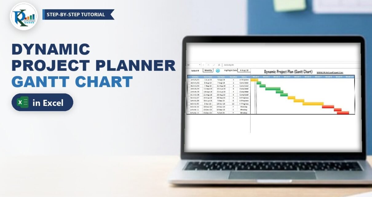
A dynamic project planner in Excel shows every activity of a project as a coloured Gantt bar and switches between a daily and a weekly timeline with one drop-down. In this tutorial you will build a project plan table, a timeline that grows or shrinks with your dates, status colours for Pending, Completed and In Progress, and a highlight line for any date. A short VBA macro redraws the chart whenever you change the view. Every step comes from PK’s original two-part video series.

Watch the Video Tutorial

Part 1 shows how the planner works and builds the table, the Daily/Weekly drop-down and the dynamic highlight-date list.

Part 2 adds the bar formula, the conditional formatting, the Refresh_Data macro and the event that switches the view automatically.

What You Will Build

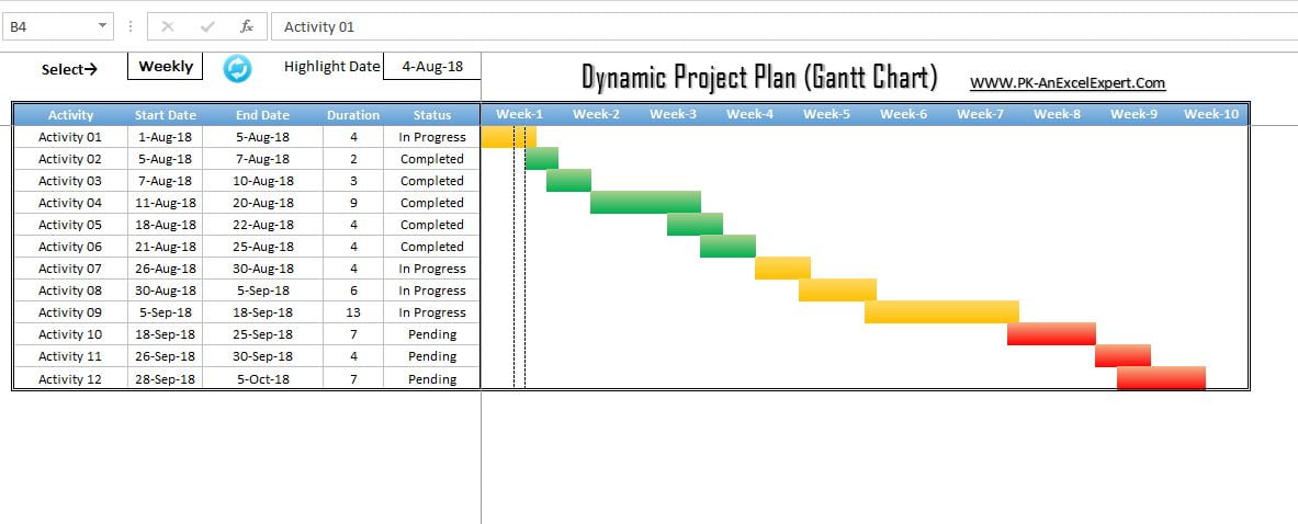
• A project plan table with Activity, Start Date, End Date, Duration and Status.
• A Gantt timeline from the earliest start date to the latest end date, with red, green and yellow bars for Pending, Completed and In Progress.
• A Daily / Weekly drop-down that redraws the timeline by day or by week.
• A highlight date shown as two dashed vertical lines.
• A protected sheet (demo password 1234).

How the Dynamic Project Planner in Excel Works

There is no chart object. Row 1 from G1 holds one hidden date per column, a formula from G4 returns each activity’s status on the days it is active, and conditional formatting turns that status into a coloured bar. The weekly view reuses the same daily cells, only narrower, under merged Week labels.

Part 1: Set Up the Project Plan Table

Step 1: Create the table

Add a new sheet and switch off gridlines with View → Gridlines. Starting in B3, type the headers Activity, Start Date, End Date, Duration and Status, then enter your activities below them (B4:F15 in the demo, Activity 01 to Activity 12, from 1-Aug-18 to 5-Oct-18). PK gives the header a two-colour blue Fill Effects gradient.

Keep columns A to F for the table and controls; the timeline always starts in column G.

Step 2: Calculate the duration

In E4 subtract the start date from the end date and fill it down:

=D4-C4

Activity 01 runs from 1-Aug-18 to 5-Aug-18, so it shows 4.

Step 3: Use only three status values

Type exactly Pending, Completed or In Progress in the Status column; the colours match on these words, so a typo means no bar.

Part 2: Add the View and Highlight Drop-downs

Step 4: The Daily / Weekly drop-down

Type Select in B1 as a label. Select C1, press Alt+D+L to open Data Validation, choose List and type the source Daily,Weekly. Pick Daily for now.

Step 5: A dynamic list of timeline dates

Type Highlight in E1. The highlight date goes in F1, and its drop-down should list only the dates currently in row 1, so you need a dynamic named range. Open Formulas → Name Manager → New, name it List and enter:

=INDIRECT("Sheet1!$G$1:"&ADDRESS(1,COUNTA(Sheet1!$G$1:$XFD$1)+6))

Replace Sheet1 with your sheet name (the finished file uses Project_Plan).

How the formula works:

• COUNTA(Sheet1!$G$1:$XFD$1) counts the dates in row 1, for example 66.
• +6 adds the six columns A to F that come before the timeline, which gives the column number of the last date.
• ADDRESS(1, ...) turns row 1 and that column number into a text address such as $BT$1.
• The text Sheet1!$G$1: is joined in front, so the result reads like Sheet1!$G$1:$BT$1.
• INDIRECT converts that text into a real range reference.

Click inside the Refers to box to check that Excel outlines the dates. Then select F1, press Alt+D+L, choose List and enter =List as the source (press F3 to paste the name).

Part 3: Draw the Gantt Bars with a Formula

Step 6: The bar formula in G4

In G4 enter:

=IF(AND($C4<=G$1,$D4>=G$1),$F4,"")

How the formula works: $C4<=G$1 checks that the activity has started by this column’s date and $D4>=G$1 that it has not ended. When both are true the cell shows the status from F4, otherwise it stays empty. $C, $D and $F lock the table columns and G$1 locks the date row, so one formula works across the whole grid.

Step 7: Colour the bars by status

Select the grid from G4 and press Alt+O+D to open the Conditional Formatting Rules Manager. Click New Rule → Format only cells that contain, choose Cell Value → equal to and type Pending. Then click Format:

• Fill → Fill Effects: Two colours, Color 1 red and Color 2 a lighter shade, horizontal shading. This gives the bars their rounded 3D look.
• Number → Custom: type three semicolons ;;;. This custom format hides the cell text, so you see only the coloured fill.

Repeat for Completed (green) and In Progress (yellow).

Step 8: Highlight the selected date

With the grid still selected (active cell G4), add one more rule: Use a formula to determine which cells to format:

=$F$1=G$1

Remove the dollar in front of G so the reference moves across the columns but stays on the date row. On the Border tab choose a dashed line and click the left and right borders: the selected date gets two dashed vertical lines.

Step 9: Keep only the formula in G4

Once the rules work, clear everything in the grid except G4. The macro fills the formula, together with its conditional formatting, across exactly the right number of rows and columns every time it runs. Finally, open Format Cells → Protection for G4 and tick Hidden.

Part 4: The VBA Macro that Switches Daily and Weekly View

Step 10: Add the Refresh_Data macro

Press Alt+F11, choose Insert → Module and paste the macro from the original workbook:

Option Explicit

Sub Refresh_Data()

Application.ScreenUpdating = False
Dim sh As Worksheet
Set sh = ThisWorkbook.Sheets("Project_Plan")
sh.Unprotect "1234"
Dim i As Long
sh.Range("G3:XFD3").UnMerge
sh.Range("G1:XFD3").Clear
sh.Range("G1:XFD3").Orientation = 0

Dim lc, lr As Integer
For i = Application.WorksheetFunction.Min(sh.Range("C:C")) To Application.WorksheetFunction.Max(sh.Range("D:D"))
    If sh.Range("G1").Value = "" Then
        sh.Range("G1").Value = i
    Else
        lc = sh.Range("XFD1").End(xlToLeft).Column
        sh.Cells(1, lc + 1).Value = i
    End If
Next i

lc = sh.Range("XFD1").End(xlToLeft).Column

If sh.Range("C1").Value = "Daily" Then
   sh.Range("G3").Value = "=G1"
   sh.Range("G3", sh.Cells(3, lc)).FillRight
   sh.Range("E3").Copy
   sh.Range("G3", sh.Cells(3, lc)).PasteSpecial xlPasteFormats
   sh.Range("G3", sh.Cells(3, lc)).NumberFormat = "D-MMM"
   sh.Range("G3", sh.Cells(3, lc)).Orientation = 90
   sh.Range("G3", sh.Cells(3, lc)).EntireColumn.ColumnWidth = 2.5
Else
    For i = 7 To lc Step 7
        sh.Cells(3, i).Value = "Week-" & i / 7
        sh.Range("E3").Copy
        sh.Range(sh.Cells(3, i), sh.Cells(3, i + 6)).PasteSpecial xlPasteFormats
        sh.Range(sh.Cells(3, i), sh.Cells(3, i + 6)).EntireColumn.ColumnWidth = 0.8
        sh.Range(sh.Cells(3, i), sh.Cells(3, i + 6)).Merge
        sh.Range(sh.Cells(3, i), sh.Cells(3, i + 6)).HorizontalAlignment = xlCenter
        sh.Range(sh.Cells(3, i), sh.Cells(3, i + 6)).VerticalAlignment = xlCenter
    Next i
    lc = sh.Range("XFD3").End(xlToLeft).Column + 6
End If

lr = sh.Range("B" & Application.Rows.Count).End(xlUp).Row
sh.Range("G1:XFD1").NumberFormat = "D-MMM-YY"
sh.Range("G1:XFD1").Font.Color = VBA.vbWhite
sh.Range("H4:XFD" & Application.Rows.Count).Clear
sh.Range("G5:G" & Application.Rows.Count).Clear
sh.Range("A" & lr + 1, "A" & Application.Rows.Count).EntireRow.Clear
sh.Range("B:F").Locked = False
sh.Range("G1:XFD3").Locked = True
sh.Range("G1:XFD3").FormulaHidden = True
sh.Range("G4:G" & sh.Range("B" & Application.Rows.Count).End(xlUp).Row).FillDown
sh.Range("G4", sh.Cells(lr, lc)).FillRight

With sh.Range("B3", sh.Cells(lr, lc))
    .Borders(xlEdgeBottom).LineStyle = xlDouble
    .Borders(xlEdgeBottom).Color = vbBlack
    .Borders(xlEdgeLeft).LineStyle = xlDouble
    .Borders(xlEdgeLeft).Color = vbBlack
    .Borders(xlEdgeRight).LineStyle = xlDouble
    .Borders(xlEdgeRight).Color = vbBlack
    .Borders(xlEdgeTop).LineStyle = xlDouble
    .Borders(xlEdgeTop).Color = vbBlack
End With

sh.Protect "1234"

End Sub

Change "Project_Plan" to your sheet name (in the video PK points it at Sheet1 while rebuilding) and "1234" to your own password, in both places.

Step 11: What the macro does

1. Reset: unprotect, unmerge the old Week headers and clear rows 1 to 3 from column G.
2. Write the dates: the For loop runs from the smallest start date in column C to the largest end date in column D and writes each date in the next free cell of row 1. Range("XFD1").End(xlToLeft) finds the last used column, like Ctrl+Left from the sheet’s right edge.
3. Daily view: G3 gets =G1 filled right, formatted D-MMM, rotated 90 degrees, columns 2.5 wide.
4. Weekly view: a loop steps seven columns at a time from column 7 (G), writes "Week-" & i / 7, makes the columns 0.8 wide and merges each block of seven.
5. Draw and protect: it hides row 1 in white font, clears old bars and rows below the table, unlocks B:F, locks and hides G1:XFD3, fills the G4 formula (with its conditional formatting) across the plan, adds a double border and protects the sheet again.

Step 12: Add a refresh button

Insert any shape or icon (PK uses a round blue refresh icon next to C1), right-click it, choose Assign Macro and pick Refresh_Data. Click it once and the timeline, the headers and the bars are created. Turn off View → Headings for a clean look.

Step 13: Refresh automatically when the view changes

So that you do not have to click the button after changing C1, add a Change event. In the VBA editor double-click the planner sheet, choose Worksheet and Change in the two drop-downs and enter:

Private Sub Worksheet_Change(ByVal Target As Range)
    If Target.Row = 1 Then
        If Target.Column = 3 Then
            Call Refresh_Data
        End If
    End If
End Sub

Row 1 and column 3 is cell C1, so the macro runs only when the Daily / Weekly choice changes. Save the workbook as .xlsm.

Using the Planner Day to Day

• Change dates or statuses, then click refresh if the project now starts earlier or ends later.
• Delete activities and refresh: in the video, removing two activities shrinks the weekly view from Week-11 to Week-9.
• Add an activity below the last row, copy the row format with the Format Painter and refresh.
• Pick a highlight date in F1; the dashed lines move in both views.

Common Errors and Fixes

Run-time error 9: Subscript out of range

The sheet name in Sheets("Project_Plan") does not match your tab name. Rename the tab or change the name in the code.

The bars show text instead of colour

The cell value does not match a rule exactly (for example “In progress” against “In Progress” with a trailing space), or the rule is missing the ;;; number format. Use a list validation on the Status column and check each rule’s format.

The highlight lines do not appear

Check that the rule formula still has the dollar on row 1 and not on column G, and that it was created with G4 as the active cell. Also make sure the date in F1 is a real date picked from the list, not text.

Tips

• In Dim lc, lr As Integer only lr is an Integer; lc becomes a Variant. It works, but Dim lc As Long, lr As Long is cleaner. (This is our addition, not part of the original video.)
• Lock the VBA project (Tools → VBAProject Properties → Protection) so users cannot read the sheet password in the code.
• Read Microsoft’s guide to using formulas with conditional formatting for more rule ideas.

Want It Ready-Made?

If you would rather start from the finished workbook, the Dynamic Project Planner Gantt Chart in Excel on NextGenTemplates.com is the exact file from this tutorial. You can also browse more Excel project management templates. To get faster with the formulas behind trackers like this one, such as IF, AND, INDIRECT and ADDRESS, take a look at the Excel + AI Mastery: 100 Essential Formulas course.

Related Tutorials

• Project Plan (Gantt Chart) in Excel
• Quick Gantt Chart in Excel
• Dynamic Hourly Project Planner (Gantt Chart)
• Power Gantt Chart Project Planner for Project Management
• Introduction to Excel VBA

Frequently Asked Questions

How do I make a Gantt chart in Excel without a chart object?

Put one date per column in a hidden row, use an IF and AND formula that returns the status when the date falls between the start and end date, and colour the cells with conditional formatting. Step 6 and Step 7 show the exact formula and rules.

How does the weekly view work?

It uses the same daily cells. The macro makes every date column only 0.8 wide and merges every seven header cells into a Week label, so seven days look like one week of the bar.

Why does the timeline not change when I edit a date?

The dates in row 1 are written by the Refresh_Data macro. Click the refresh button after changing the project start or end so the timeline is rebuilt. Changing C1 runs the macro automatically through the Worksheet_Change event.

Can I change the status colours?

Yes. Unprotect the sheet, open Conditional Formatting, Manage Rules for the grid and edit the Fill Effects colours of each status rule. Keep the three-semicolon number format so the text stays hidden.

Does the planner work without macros?

The bars and colours are formulas and conditional formatting, so they still display. But switching views and extending the timeline need the macro, so save the file as .xlsm and enable macros.

About the Author

PK is a Microsoft Excel expert and trainer and the founder of PK: An Excel Expert and NextGenTemplates.com. He has been teaching Excel, VBA, Power Query and Power BI since 2016 on his YouTube channel.

Conclusion

A dynamic project planner in Excel needs three ingredients: an IF and AND formula that marks the active days, three conditional formatting rules that turn statuses into coloured bars, and a Refresh_Data macro that writes the dates and switches between daily and weekly views. Add the highlight date and protection, and your Gantt chart keeps up with the project.