Quick Gantt Chart

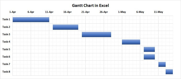
In this article you will learn how we can create a Gantt Chat quickly in Microsoft Excel. A Gantt Chart is used to show the project plan or project schedule. We will create this chart by using the horizontal Stacked Bar Chart. Position of the bar will display the Start Date of an activity. Length of the bar will display the duration of the activity.

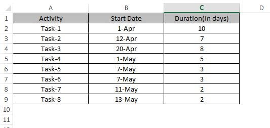
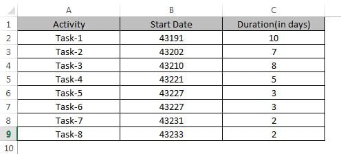
Below is the data set for which we will create the Gantt Chart. In this table there are 8 activities/tasks, their start date and duration(in days).

Table of Contents

Below are the step to create a Quick Gantt Chart in Excel

Select the column B in the date set and change the format as General (Press Shift+Ctrl+~)

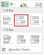
Select the entire data set and go to Insert Tab>>Charts>>Insert 2D Bar Chart.

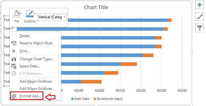
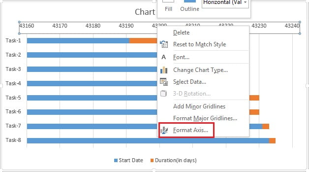
In the Bar Chart Right click on the Vertical Axis (Task names) and click on Format Axis.

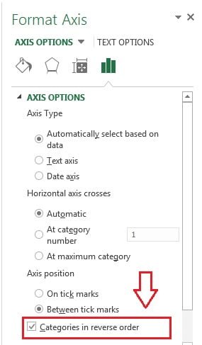
In the Format Axis window, tick the Categories in reverse order.

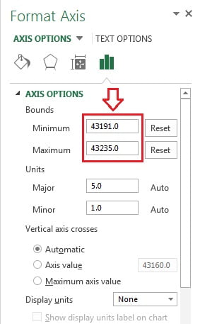
Now right click on Horizontal Axis (on dates) and click on Format Axis.

Put the Minimum value as “43191” (Start date of Task-1)
Put the Maximum value as “43235” (Start date of Task-8 + Duration of Task-8)

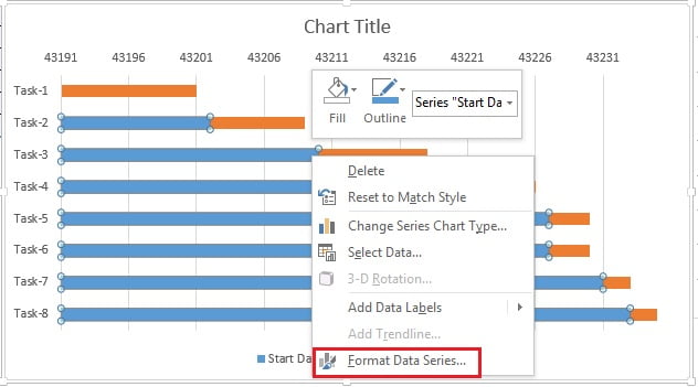
Now in the chart select the blue bars (Start Date series)
Right click and click on Format Data Series.

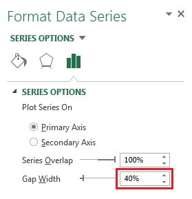
In Format Data Series window, select Gap Width as 40% available under Series Option.

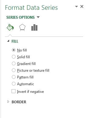
In Format Data Series window, select the Fill & Line option.
Select No fill option available in under Fill.

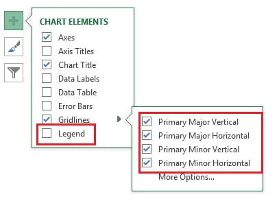
Click on Chart Elements button (“+” button of chart)
Remove the Legend and tick all the Gridlines.

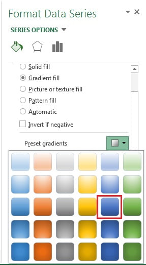
Now select the orange bar and right click and click on Format Data Series.
In Format Data Series window go to the Fill & Line option.
Select the Gradient fill option available under Fill.
Select a Preset gradients as given in below image.

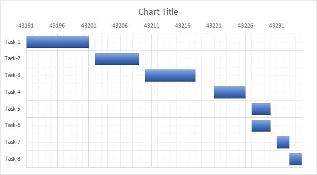
After doing the above settings, our chart will look like below image.

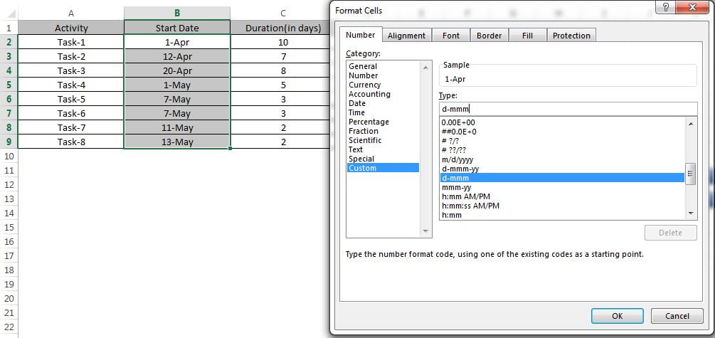
Now select the column B in data set can open Format cells window by using Shortcut key Alt+O+E.
Go to the Custom in Number tab and give the Type as “d-mmm“