Circle Invalid Data in Excel: Find Entries That Break Validation

Part of the free Module 6: Data Validation · Lesson 10 of 14 · Full Excel course

Updated on 5 September 2026 · Works in Excel 365, 2021, 2019 and 2016 for Windows and Mac. Not available in Excel for the web.

Circle Invalid Data in Excel is a Data Validation command that draws a red oval around every cell whose current value breaks its validation rule. Data validation only checks values as they are typed, so anything entered before the rule, pasted in, filled down or produced by a formula slips through. Circle Invalid Data audits those cells after the fact so you can fix them and clear the circles.

Why a validated cell can still hold an invalid value

Many people assume that once a rule is set, the range is clean. It is not. Validation runs only when a value is committed by typing in the cell and pressing Enter. Every other way of getting a value into a cell bypasses the rule completely. The table below lists the usual causes, with the fix for each.

Why the value is invalid	What happened	Fix
Typed before the rule existed	The data was entered first and the rule was added later; Excel never re-checks old values.	Run Circle Invalid Data and correct the circled cells.
Pasted or filled in	Paste, Ctrl+D, the fill handle and Flash Fill write values without validation. A plain paste also overwrites the rule itself.	Use Paste Special > Values, then circle and fix. Re-apply the rule if it was overwritten.
Formula result	A formula in a validated cell can return any value; rules apply to typed entries, not to calculated results.	Move the formula out of the validated range or audit it with a helper column.
Rule edited later	The limits were tightened (for example 18 to 65 instead of 0 to 120) after the data was entered.	Circle Invalid Data immediately after changing any rule.
Warning or Information alert	The Error Alert style lets the user click Yes or OK and keep the wrong value.	Circle to find them, then consider switching the alert to Stop.
Macro or external import	VBA, Power Query and linked data write directly into cells.	Add a validation check to the import step or audit with a formula.

Step by step: circle invalid data in an existing range

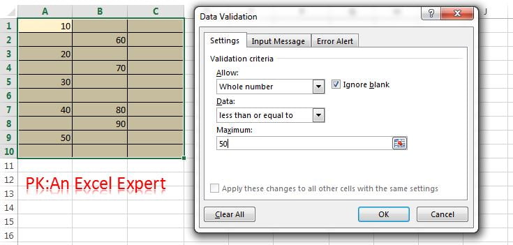
1. Start with a range that already holds numbers, as in the screenshot below. Select it and go to Data > Data Tools > Data Validation. Apply a Whole number rule with Data: less than or equal to and Maximum: 50, then click OK.

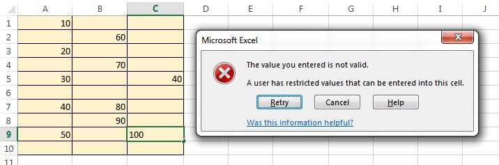
2. From now on, typing a number greater than 50 is rejected with the Stop alert. The values above 50 that were already in the cells stay exactly where they are, and they are now invalid according to the rule.

3. Click any cell on the sheet. The command checks every validated cell on the active worksheet, so the selection does not matter.
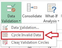
4. Go to Data > Data Tools > Data Validation, click the small arrow under the button and choose Circle Invalid Data.

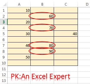
5. Every cell that fails its rule is circled in red. Correct the values one by one. A circle disappears the moment its cell becomes valid, so the sheet is clean when no circles are left.

Clear the validation circles

1. Go to Data > Data Validation, open the drop-down and click Clear Validation Circles. Do this once you have fixed the entries, or when you want a clean view for a screenshot or a review meeting.

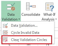
The circles are temporary drawing objects, not cell formatting. They are not stored with the workbook, so in most versions they vanish when you save or close the file, and they do not print reliably. Treat them as a review tool, not as a record.

Limits of Circle Invalid Data

• 255 circles per sheet. Excel stops drawing after 255 cells. Fix or filter those, clear the circles and run the command again for the rest.
• Active sheet only. Repeat the command on every sheet that carries validation.
• Blanks are skipped. A cell left empty is not circled while Ignore blank is ticked in the rule. Untick it if empty cells must be flagged.
• Nothing to compare to. Custom rules that refer to other cells are evaluated with the current values of those cells, so a circle can appear or disappear when unrelated data changes.
• Desktop only. Excel for the web still enforces rules on new entries but has no Circle Invalid Data command.

Permanent alternatives: helper column, conditional formatting and counts

For a recurring audit you need something that stays on the sheet. Three approaches work everywhere from Excel 2016 onwards. The next section shows them on real data; this table summarises when to pick each.

Method	How it works	Best for	Drawback
Circle Invalid Data	Built-in command; draws red ovals around failing cells on the active sheet.	A quick one-off check after import or after adding a rule.	Temporary, 255-cell limit, not printed, not in Excel for the web.
Helper column	A logical formula next to the data returns TRUE or FALSE for each row.	Filtering, sorting and counting the failures; auditing formula results.	Needs a spare column; the formula must mirror the rule exactly.
Conditional formatting	The same formula as a rule under Home > Conditional Formatting > New Rule.	A permanent visual flag that prints and survives saving.	Formatting only; cannot be filtered without a helper column.
COUNTIF or SUMPRODUCT	One formula that counts how many entries break the rule.	A dashboard-style health check or a sign-off cell.	Tells you how many, not which.

To find which cells carry a rule at all, use Home > Find & Select > Go To Special > Data validation > All. This selects every validated cell on the sheet, which is the quickest way to confirm that a rule was not lost by a careless paste.

Worked example: adding an age rule to 20 existing entries

A registration list in A2:A21 was typed months ago with no rule. You now add a Whole number rule, between 18 and 65, to the whole range. The data looks like this:

Rows 2 to 6	Rows 7 to 11	Rows 12 to 16	Rows 17 to 21
23	52	15.5	58
45	29	60	65
17	70	27	18
31	38	33	44
66	41	19	N/A

1. Select A2:A21, open Data > Data Validation, choose Allow: Whole number, Data: between, Minimum 18, Maximum 65, and click OK. No message appears; the old values are untouched.
2. Click Data Validation > Circle Invalid Data. Five cells are circled: 17 (below 18), 66 and 70 (above 65), 15.5 (not a whole number) and N/A (text). The boundary values 18 and 65 are valid because between is inclusive.
3. Fix each cell. Replace 17 with the correct age or move the record to a minors list, correct 66 and 70 or raise the limit if the policy allows, round 15.5 to a whole number after checking the source, and replace N/A with a real value or leave the cell blank (blank passes while Ignore blank is ticked). Each circle disappears as you press Enter.
4. Click Clear Validation Circles if any remain, for example after you decide to keep a value.

For a permanent check, put this in B2 and fill down to B21:

=IFERROR(AND(ISNUMBER(A2), MOD(A2,1)=0, A2>=18, A2<=65), FALSE)

The formula returns TRUE for a valid age and FALSE for the same five cells that Excel circled. The IFERROR wrapper stops text such as N/A from producing #VALUE!. Count the failures with =COUNTIF(B2:B21,FALSE), which gives 5. To skip the helper column entirely, use a single count:

=SUMPRODUCT(--NOT(IFERROR(ISNUMBER(A2:A21)*(MOD(A2:A21,1)=0)*(A2:A21>=18)*(A2:A21<=65),0)))

To highlight the failures permanently, select A2:A21, go to Home > Conditional Formatting > New Rule > Use a formula and enter =NOT(IFERROR(AND(ISNUMBER(A2), MOD(A2,1)=0, A2>=18, A2<=65), FALSE)) with a red fill. This flag prints, survives saving and has no 255-cell limit.

Tips and common mistakes

• Circle straight after applying a rule to old data. Make it a habit: apply, circle, fix, clear. The rule alone never touches existing values.
• Circle after every paste. A plain paste replaces both the value and the validation rule. Use Paste Special > Values to keep the rule, then circle to check the new values.
• Do not rely on circles for sign-off. They are not saved and rarely print. Use a helper column or a COUNTIF so the audit is visible in the file.
• Remember the 255 limit. If exactly 255 cells are circled, there are almost certainly more. Fix, clear and run again.
• Check Ignore blank. With the box ticked, empty cells and cells that reference an empty named range are never circled.
• Match the helper formula to the rule. A Whole number rule needs the MOD(A2,1)=0 test; a Decimal rule does not. A Date rule should test with ISNUMBER and the date limits.
• Change Warning alerts to Stop where it matters. If circles keep reappearing in the same column, the rule is letting values through. See the Error Alert lesson.

Errors and how to fix them

Symptom	Cause	Fix
Circle Invalid Data does nothing	No cell on the active sheet has validation, or every value passes.	Use Go To Special > Data validation to confirm rules exist; check the rule limits.
Command is greyed out	The sheet is protected or the workbook is in Protected View.	Unprotect the sheet or click Enable Editing.
Only some invalid cells are circled	The 255-circle limit was reached.	Fix the first batch, clear, and run again.
A blank cell is not circled	Ignore blank is ticked in the rule.	Untick it, or add a helper column that tests for empty cells.
Circles vanished after reopening	Circles are not saved with the file.	Run the command again or switch to conditional formatting.
Helper formula returns #VALUE!	Text in the data hits MOD or a comparison.	Wrap the AND in IFERROR(…,FALSE) as shown above.

Practice exercise

1. Type any 15 numbers between 1 and 100 in A1:A15. Then add a Whole number rule between 10 and 50 and circle the invalid entries. Count the circles.
2. Copy a value of 500 into three of the cells with plain paste. Circle again and note that the pasted cells are no longer circled: check with Go To Special > Data validation which cells lost the rule.
3. Build the helper column from the worked example for your 15 numbers and confirm that =COUNTIF(B1:B15,FALSE) matches the number of circles.
4. Replace the helper column with a conditional formatting rule using the same formula, save the file, reopen it and confirm that the highlighting is still there while the circles are gone.

Key takeaways

• Data validation checks typed entries only; existing, pasted, filled and calculated values are never re-checked.
• Data > Data Validation > Circle Invalid Data marks every failing cell on the active sheet with a red oval, up to 255 at a time.
• Circles are temporary: they clear when the cell is fixed, with Clear Validation Circles, and usually on save or close.
• The reliable workflow is apply the rule, circle, fix, clear.
• For a permanent audit, mirror the rule in a helper column, a conditional formatting rule or a COUNTIF/SUMPRODUCT count.

Related lessons

• Data Validation course hub
• Whole number data validation
• Error alert: Stop, Warning and Information
• Copy, find and remove data validation with Go To Special
• Conditional formatting with a formula
• COUNTIF function
• Microsoft Support: Apply data validation to cells

Visit our YouTube channel for step-by-step video tutorials.

Frequently asked questions

Why does Excel show invalid data even though I set a validation rule?

Validation only runs when a value is typed into the cell. Values that were there before the rule, values pasted or filled in, formula results and entries accepted through a Warning or Information alert are never checked. Run Data > Data Validation > Circle Invalid Data to find them, then fix the circled cells.

Why does Circle Invalid Data show nothing?

Either every validated cell passes its rule, or no cell on the active sheet carries validation. Use Home > Find & Select > Go To Special > Data validation to select all validated cells. If nothing is selected, the rule was lost, often because a plain paste replaced it.

Do the validation circles stay when I save or print the workbook?

No. The circles are temporary drawing objects that are not stored in the file and do not print reliably. They also disappear when a cell is corrected or when you click Clear Validation Circles. For a permanent, printable flag, use a conditional formatting rule built on the same logic as the validation rule.

Is there a limit to how many cells Circle Invalid Data can mark?

Yes. Excel draws at most 255 circles on a sheet in one run. If your data has more failures, fix or filter the first 255, clear the circles and run the command again. A helper column with a logical formula has no such limit and can be filtered to show only the failures.

Can I circle invalid data in Excel for the web or with a formula?

Excel for the web enforces rules on new entries but has no Circle Invalid Data command. Use a helper column instead, for example =AND(ISNUMBER(A2),A2>=18,A2<=65), and count the FALSE results with COUNTIF. The same formula works in every desktop version as a permanent audit.

Want the finished version? Ready-made Excel dashboards, trackers and VBA systems are available at NextGenTemplates.com.