In this video, we have explained how to create a Quick Weekly Attendance Template in Excel using New Check box feature in office 365 and Conditional formatting.
Follow the below given step to achieve this-
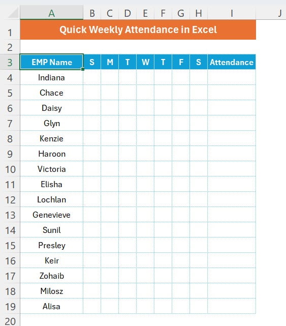
Put the headers:
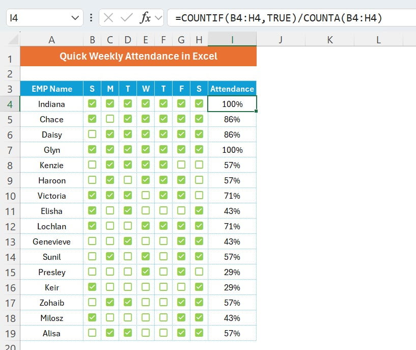
Add the headers first from Range A3 to I3 as given below
- Emp Name on A3
- First letter of the day as S, M, T, W, T, F and S on range B3 to H3
- Put “Attendance” on range I3
Enter Emp Names:
Put the Employee name on from range A4. We have put here Emp Name from range A4 to A19.
Insert check boxes:
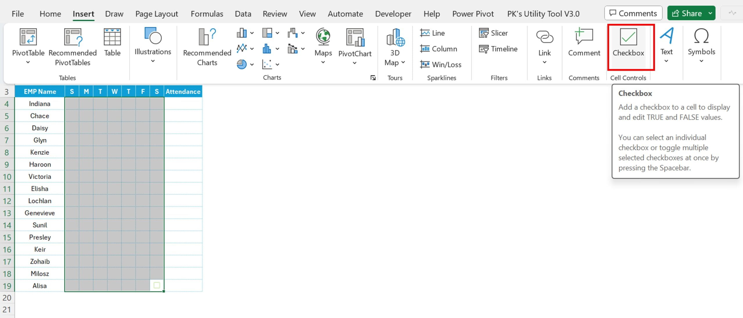
- Select the range B4:H19
- Go to insert and insert the check box
- Take the font size as 8
- Reduce the column width as 2.5 or 3
- Take the font color as light green
Put the Attendance Formula:
- Put the formula on range I4 as “=COUNTIF(B4:H4,TRU/COUNTA(B4:H4)”
- Fill this down from I4 till I19
- change into percentage format using shortcut key Shift+Ctrl+5
Add Conditional Formatting Data Bar:
- Select the range I4:I19
- Press Alt +O+D to open the Conditional Formatting Rule Manager.
- Click on New Rule
- Select Format Style as “Data Bar”
- Select Minimum and Maximum Type as Number.
- Take Minimum Value as 0 and Maximum value as 1
- Select Gradient Fill in Fill.
- Choose Color as orange.
- Choose Solid Border in Border and Border color as Orange.
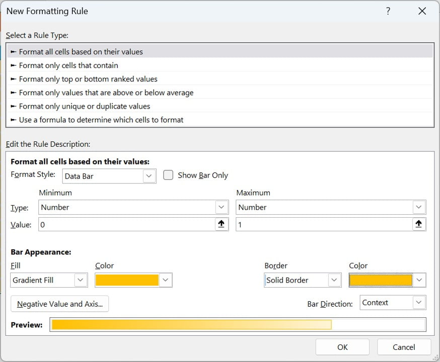
- Click on OK and Apply the Rule.
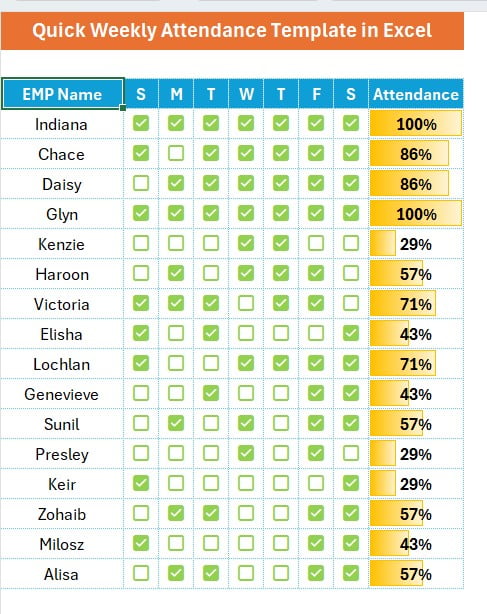
Our Quick Weekly Attendance Template in Excel is ready to use.
Visit our YouTube channel to learn step-by-step video tutorials
Watch the step-by-step video tutorial:
Click here to download the practice file
Want the ready-made Weekly Attendance Sheet in Excel?
Skip the build and get the finished, fully working template, ready to use with your own data.
Want to master these skills step by step? Join the video course Excel + AI Mastery: 100 Essential Formulas and Real-World Projects.