Part of the free Module 3: Find and Replace · Lesson 3 of 6 · Full Excel course
Updated on 5 September 2026 · Works in Excel 365, 2021, 2019 and 2016 unless noted.
Find and replace formatting in Excel uses the two Format buttons in the Find and Replace dialog. The first finds every cell with a given fill colour, font, number format or border; the second applies a new format to each match. Leave the Find what and Replace with boxes empty and Excel changes only the formatting, never the values.
Where the Format buttons are
Press Ctrl+H and click Options >>. A Format… button appears to the right of Find what and another to the right of Replace with. Each button has a small arrow with three choices:
- Format… opens the Find Format (or Replace Format) dialog with the familiar Number, Alignment, Font, Border, Fill and Protection tabs.
- Choose Format From Cell… turns the pointer into an eyedropper. Click any cell and Excel copies every format attribute of that cell into the search.
- Clear Find Format (or Clear Replace Format) removes the format condition. A preview box between the Find what box and the button shows “Preview” with the chosen look, or “No Format Set”.
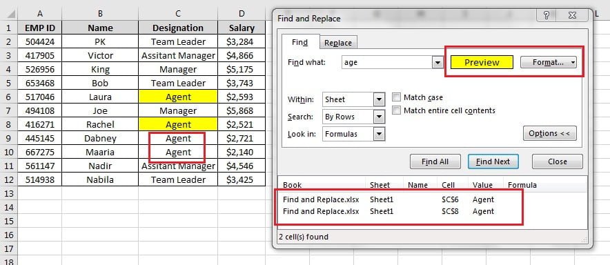
Find and count cells with a specific colour
- Select the range, or one cell for the whole sheet, and press Ctrl+F. Click Options >>.
- Click the arrow on Format and choose Choose Format From Cell, then click a cell that has the colour you want.
- Leave Find what empty and click Find All. The bottom of the list shows “n cell(s) found”.
- Press Ctrl+A inside the list to select every coloured cell. The status bar now shows Count and, for numbers, Sum and Average.
This is the quickest honest way to count or sum coloured cells without VBA. Because the eyedropper copies the font, borders and number format too, open Format… afterwards and clear the tabs you do not care about, otherwise a cell with the right fill but a different font is skipped.
Replace one fill colour with another
- Press Ctrl+H and click Options >>.
- Next to Find what, choose Format… > Fill, click the old colour and press OK.
- Next to Replace with, choose Format… > Fill, click the new colour and press OK.
- Leave both text boxes empty. Set Within to Workbook if the colour is used on several sheets.
- Click Replace All. Excel reports the number of cells re-coloured; their values and formulas are untouched.
Replace fonts, bold and number formats
The same steps work for any attribute in the Find Format dialog. Three common jobs:
- Turn every bold red cell into regular black text. Find Format: Font tab, Bold, colour red. Replace Format: Font tab, Regular, colour Automatic.
- Change a date format everywhere. Find Format: Number tab, Date, the current style. Replace Format: Number tab, Date, the new style. Only cells formatted with exactly that style are matched.
- Reset cells formatted as Text. Find Format: Number tab, Text. Replace Format: Number tab, General. The format changes, but a value stored as text stays text until you re-enter it, run Data > Text to Columns > Finish or multiply by 1 with Paste Special.
Cell styles and the styles gallery
Cells formatted with a named style (Home > Styles, such as Input, Calculation or Heading 1) can be found through their underlying attributes, but Find Format has no “style name” box. To change every cell that uses a style, do not use Find and Replace at all: right-click the style in the gallery, choose Modify and edit it. Every cell carrying that style updates at once, which is exactly what styles are for.
What Find Format can and cannot match
| Format | Found by Find Format? | Alternative |
|---|---|---|
| Fill colour applied directly | Yes | Sort or Filter by Colour |
| Font colour, bold, italic, size | Yes | – |
| Number format (dates, currency, Text) | Yes | Go To Special > Constants > Text for text-numbers |
| Alignment, borders, wrap text | Yes | – |
| Protection: Locked or Hidden | Yes | – |
| Colour from a conditional formatting rule | No | Go To Special > Conditional formats, or Manage Rules |
| Data bars, colour scales, icon sets | No | Conditional Formatting > Manage Rules |
| Banding from a Table style | No | Table Design > Table Styles |
| Named cell style | Only by its attributes | Modify the style in the gallery |
Worked example: recolour overdue invoices
| Invoice | Customer | Days overdue | Fill |
|---|---|---|---|
| 1041 | PK Traders | 0 | None |
| 1042 | Victor Ltd | 18 | Red |
| 1043 | King Stores | 45 | Red |
| 1044 | Laura and Co | 3 | None |
The finance team wants overdue rows in amber instead of red, and the bold customer names set back to regular.
- Select A2:D5 and press Ctrl+H, then Options.
- Find what Format: Fill, red. Replace with Format: Fill, amber. Replace All reports 8 cells (two rows of four).
- Click both Clear Find Format and Clear Replace Format.
- Find what Format: Font, Bold. Replace with Format: Font, Regular. Replace All reports 4 cells.
Every value, including the invoice numbers, is exactly as before.
Tips and common mistakes
- Clear the format when you finish. The Find Format stays set for the whole Excel session and silently filters every later search.
- The eyedropper copies everything. Choose Format From Cell picks up font, borders and number format as well as the fill. Open Format… and clear the tabs you do not need.
- Conditional colours are invisible to Find Format. If a cell looks red because of a rule, search for the rule with Go To Special instead.
- Theme colours and standard colours are different values. A red picked from the theme row does not match a red picked from Standard Colors, even if they look alike.
- Empty Find what plus a Replace format rewrites every matched cell. Always set a Find format too, or select a range first.
- Replacing a number format does not convert the data. Text numbers need re-entry, Text to Columns or VALUE.
- Undo works. One Ctrl+Z reverses a whole Replace All.
Errors and how to fix them
| Symptom | Cause | Fix |
|---|---|---|
| “We couldn’t find what you were looking for” although the colour is visible | The colour comes from conditional formatting or a table style, or the eyedropper also captured a font that differs | Use Go To Special > Conditional formats; or open Format… and clear the Font and Border tabs |
| Plain text search suddenly finds nothing | A Find Format is still set from earlier | Format > Clear Find Format |
| Wrong cells changed colour | Find what was empty and no Find Format was set, so every cell in the selection matched | Ctrl+Z, set a Find Format before Replace All |
| Dates still show the old style | The cells use a custom format that is not identical to the one searched | Use Choose Format From Cell on one of the actual cells |
Practice exercise
- In the practice file, fill every Agent row in yellow by hand, then use Find All with Choose Format From Cell to count them.
- Replace the yellow fill with light green across the sheet without typing anything in Find what or Replace with.
- Make the Salary column bold, then use Find and Replace Formatting to set it back to regular.
- Format the EMP ID column as Text, then find those cells by number format and replace the format with General.
- Add a conditional formatting rule that colours salaries above 5,000, then confirm Find Format cannot find them and Go To Special can.
Key takeaways
- Options >> reveals a Format button beside Find what and beside Replace with.
- Empty text boxes plus two formats replace formatting only; values stay intact.
- Find All followed by Ctrl+A counts and selects every coloured cell.
- Find Format cannot see conditional formatting or table-style colours.
- Clear Find Format after each job or later searches fail.
- To change a named style everywhere, modify the style rather than searching.
Related lessons
- Find and Replace in Excel: the complete guide (module hub)
- Go To Special: select blanks, formulas and visible cells
- Find and Replace wildcards: 10 patterns
- Find and replace across sheets and workbooks
- Conditional Formatting course
- Manage and clear conditional formatting rules
- Sort by colour in Excel
- Microsoft Support: Find or replace text and numbers on a worksheet
Frequently asked questions
How do I find all cells with a specific colour in Excel?
Press Ctrl+F, click Options, then use the Format button’s Choose Format From Cell option and click a cell with that colour. Leave Find what empty and click Find All. Every cell with the same fill is listed, with the count at the bottom, and Ctrl+A in the list selects them all on the sheet.
How do I replace one cell colour with another in Excel?
Press Ctrl+H and click Options. Set the Format next to Find what to the old fill colour and the Format next to Replace with to the new colour. Leave both text boxes empty and click Replace All. Excel changes only the fill; the numbers, text and formulas in those cells are untouched.
Why does Find Format not find my conditionally formatted cells?
Conditional formatting is applied on top of the cell’s own format, and Find Format reads only the cell’s own format. Select the cells and use Go To Special, Conditional formats to find them, or open Conditional Formatting, Manage Rules to see where each rule applies and edit its colour there.
Can I count coloured cells with Find and Replace?
Yes. Find All with a Find Format set lists every matching cell and shows “n cell(s) found”. Press Ctrl+A inside the list and the status bar reports Count, Sum and Average for the selection. For a formula that updates automatically you need VBA or a helper column, because Excel has no built-in COUNTBYCOLOR function.
Does replacing the number format convert text to numbers?
No. Replacing the Text format with General changes how future entries are treated, but existing values stored as text stay text. After changing the format, select the column and run Data, Text to Columns, Finish, or paste a 1 with Paste Special, Multiply, to convert them to real numbers.
Want the finished version? Ready-made Excel dashboards, trackers and VBA systems are available at NextGenTemplates.com.