In the competitive landscape of today’s business world, tracking and analyzing key performance indicators (KPIs) is vital for assessing and improving your organization’s performance. Microsoft Excel provides various functions to simplify this task, and in this all-inclusive guide, we’ll focus on building a dynamic KPI indicator utilizing the SEQUENCE and CEILING functions in Excel. Additionally, we’ll discuss the benefits of using these functions and address some common questions.
Defining KPI Indicators
A KPI indicator is a visual representation of a key performance indicator value in Excel. KPIs are quantifiable values that enable organizations to monitor their progress towards achieving specific objectives. By employing KPI indicators in Excel, businesses can evaluate their performance and make well-informed decisions based on the data.
Comprehending the SEQUENCE and CEILING Functions in Excel
To develop a dynamic KPI indicator, it’s crucial to grasp the SEQUENCE and CEILING functions in Excel. These functions offer a robust method for creating dynamic KPI indicators that can adjust to data changes.
Introducing the SEQUENCE Function
The SEQUENCE function generates a sequence of numbers in an array. Here’s a quick summary of its features:
Description:
Produces a sequence of numbers in an array, like 1, 2, 3, 4.
Syntax:
=SEQUENCE(rows, [columns], [start], [step])
Arguments:
- Rows (required): The number of rows to return.
- [columns] (optional): The number of columns to return.
- [start] (optional): The first number in the sequence.
- [step] (optional): The increment for each subsequent value in the array.
Notes: Optional arguments default to 1 if omitted. You must provide at least one other argument if you omit the rows argument.
Introducing the CEILING Function
The CEILING function rounds up a number to the nearest multiple of significance. Here’s a quick summary of its features:
Description:
Rounds up a number, away from zero, to the nearest multiple of significance.
Syntax:
=CEILING(number, significance)
Arguments:
- Number (required): The value you want to round.
- Significance (required): The multiple to which you want to round.
Notes: If either argument is nonnumeric, CEILING returns the #VALUE! error value.
KPI Indicator with SEQUENCE and CEILING Functions in Excel – Step by Step Guide
With an understanding of the SEQUENCE and CEILING functions, let’s create a KPI indicator using these functions in Excel. Follow these steps:
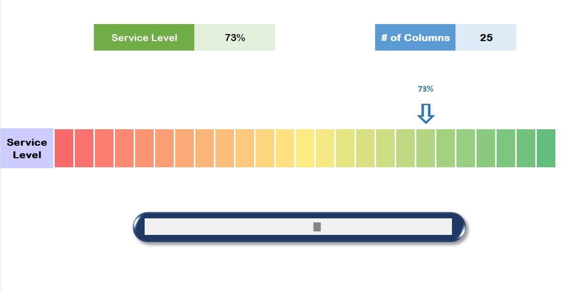
- Place the Service Level value and the number of columns in cell I5 and column V5, respectively. Name these two cells KPI_value and NumberOfColumns.
- In row number 10, create the KPI indicator. In cell A10, insert the “Service Level” text or any other KPI name.
- Adjust the column width for columns B to AO to 3 points.
- In cell B10, use the following formula:
=SEQUENCE(1, NumberOfColumns)
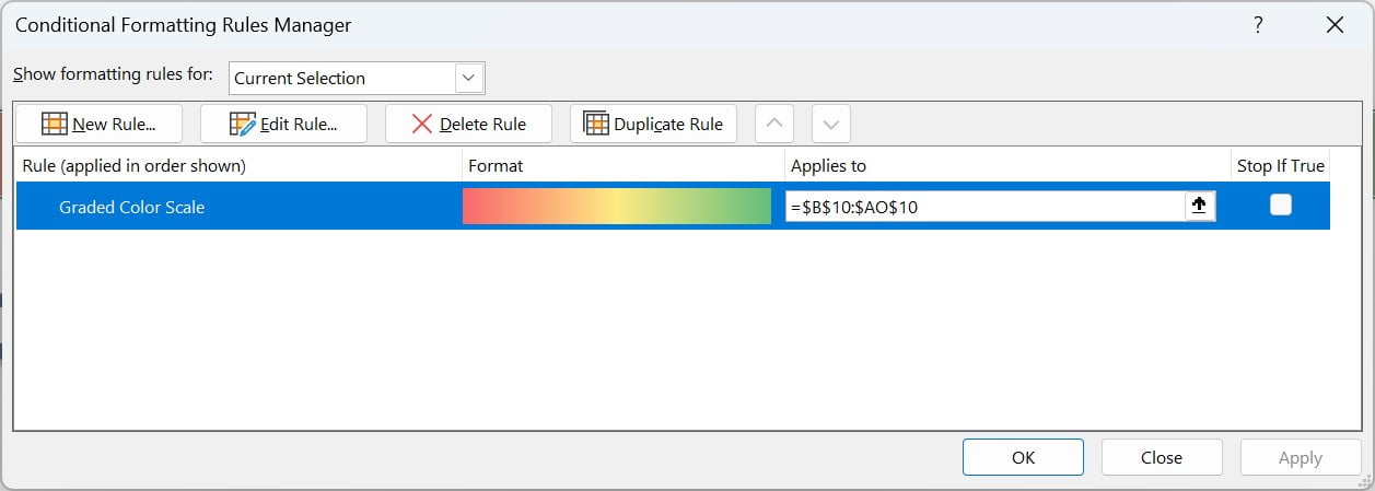
- Apply the graded color scale conditional formatting with red, yellow, and green colors to the range B10:AO10.
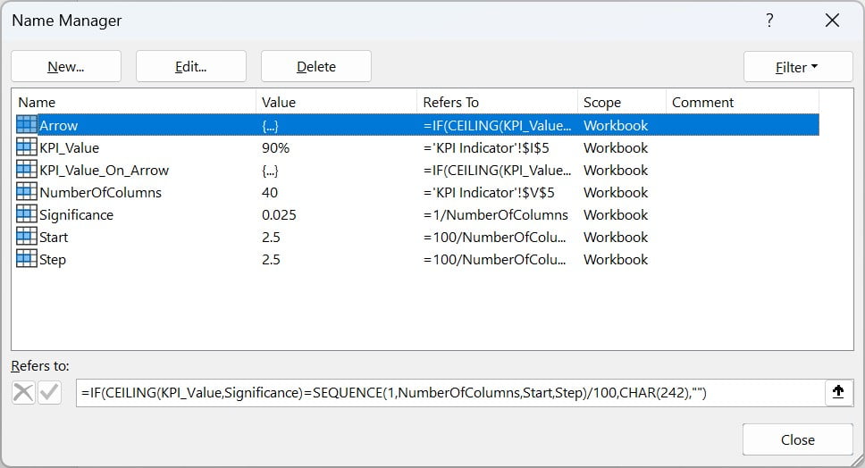
- Create the following named formulas:
- Start = 100 / NumberOfColumns
- Step = 100 / NumberOfColumns
- Significance = 1 / NumberOfColumns
- Arrow = IF(CEILING(KPI_Value, Significance)=SEQUENCE(1, NumberOfColumns, Start, Step)/100, CHAR(242), “”)
- KPI_Value_On_Arrow = IF(CEILING(KPI_Value, Significance)=SEQUENCE(1, NumberOfColumns, Start, Step)/100, KPI_Value, “”)
named formulas
- In cell B9, use the following formula:
=Arrow
- Change the font of the range B9:AO9 to “Wingdings” with a font size of 36.
- In cell B8, use the following formula:
=KPI_Value_On_Arrow
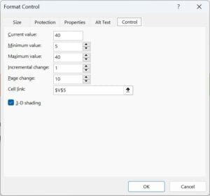
- Insert a Form Control Scroll Bar by navigating to the Developer tab >> Insert >> Form Control Scroll Bar.
- Right-click on the scroll bar and select “Format Control.” In the Format Control window, set the following values:
- Minimum Value: 5
- Maximum Value: 40
- Cell Link: $V$5
Now, your KPI indicator chart is ready for use.
Benefits of Employing SEQUENCE and CEILING Functions for KPI Indicators in Excel
Several advantages come from using SEQUENCE and CEILING functions for creating KPI indicators in Excel:
Dynamic KPI Indicators:
Firstly, these functions enable you to build dynamic KPI indicators that automatically adapt to data changes, making it simpler to examine trends and performance over time.
Enhanced Visualization:
Secondly, the combination of these functions allows you to create visually appealing KPI indicators, making it easier to understand the data and identify patterns.
Customizable:
Thirdly, the KPI indicator created using SEQUENCE and CEILING functions can be easily tailored to meet your specific needs or preferences, making it a versatile solution for various applications.
Time-Saving:
Lastly, these functions help you create KPI indicators quickly and efficiently, saving time and effort compared to manual methods.
Frequently Asked Questions
Q. Is it possible to utilize other Excel functions for crafting KPI indicators?
Absolutely! You can choose from a variety of Excel functions to create KPI indicators. Indeed, the most suitable functions will depend on your specific requirements and the intricacy of the data you’re dealing with.
Q. How can I modify the KPI indicator’s appearance to my liking?
A. To personalize the look of your KPI indicator, you can adjust the font, colors, conditional formatting, and other available formatting options in Excel. Furthermore, experimenting with different styles will help you achieve your desired appearance.
Q. Can this approach be applied to generate KPI indicators for various data types?
Yes, indeed! You can adapt the method outlined in this guide to develop KPI indicators for a wide range of data types. Consequently, to fit your specific needs, you might need to alter the formulas and formatting settings.
Q. Do SEQUENCE and CEILING functions offer any advantages when creating KPI indicators?
Utilizing the SEQUENCE and CEILING functions in Excel comes with multiple benefits, such as dynamic and visually appealing KPI indicators, customization, and time-saving capabilities. Thus, incorporating these functions into your analysis can greatly improve your overall experience.
Conclusion
In conclusion, the SEQUENCE and CEILING functions in Excel provide a powerful and flexible way to create dynamic KPI indicators that can help organizations track their performance and make informed decisions. Moreover, by following this guide, you can create a visually appealing and customizable KPI indicator that will undoubtedly enhance your data analysis capabilities.
Visit our YouTube channel to learn step-by-step video tutorials