Excel's Conditional Formatting Magic!

Table of Contents

Introduction

Welcome to our deep dive into one of Excel’s most powerful features – Conditional Formatting. This tool isn’t just a feature; it’s a magic wand in your Excel arsenal, especially when dealing with extensive data sets. Today, we’re translating our popular YouTube video, “Excel’s Conditional Formatting Magic!”, into a comprehensive guide.

Understanding the Basics

Firstly, let’s clarify what Conditional Formatting in Excel is all about. It’s a fantastic way to visually highlight data based on certain criteria. Think of it as Excel’s way of saying, “If this condition is true, then make the data look like this!”

The COUNTIF Function: Your Key to Conditional Formatting

Now, let’s delve into the core of our video: using the COUNTIF function in Conditional Formatting. Why COUNTIF, you might ask? It’s simple yet powerful. COUNTIF allows you to count the number of times a specific condition is met within a range. In our case, we’re interested in highlighting unmatched entries.

Practical Application: Employee Sales Data

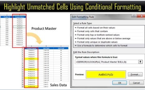
Imagine you have a dataset with employee sales details from A2 to B17 and a separate list of employee names from E1 to E18. Our goal is to identify and highlight any employee names in our sales data that don’t appear in our employee list.

The Magic Formula: =COUNTIF($E$2:$E$18,A2)=0

Here’s where the magic happens. We apply this formula as a Conditional Formatting rule to the range A2:A17. What does this formula do? It checks each name in our sales data against the employee list. If a name doesn’t appear in the employee list, COUNTIF returns 0, triggering our formatting rule.

Visual Impact: Highlighting with Yellow

To make these unmatched entries stand out, we’ve chosen to highlight them in yellow. This visual cue is not only eye-catching but also immensely helpful in quickly identifying discrepancies in our data.

Wrapping Up: The Power of Conditional Formatting

In conclusion, Conditional Formatting, especially when paired with functions like COUNTIF, is a game-changer in Excel. It not only adds visual clarity to your data but also enhances your ability to spot anomalies and trends swiftly.

Next Steps: Practice and Explore

Now that you’ve grasped the concept, it’s your turn to try it out. Experiment with different conditions and formatting styles. Remember, Excel’s Conditional Formatting is a tool limited only by your imagination!