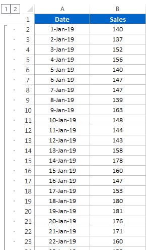
In this article, we have explained Excel formula and Linear Regress to forecast sales in upcoming month. We have used 1st Jan 2019 to 31st Mar’19 sales data to do the Forecasting in Excel for Apr’19.
Forecasting in Excel
We have used for different method to do the forecasting-
Forecast formula:
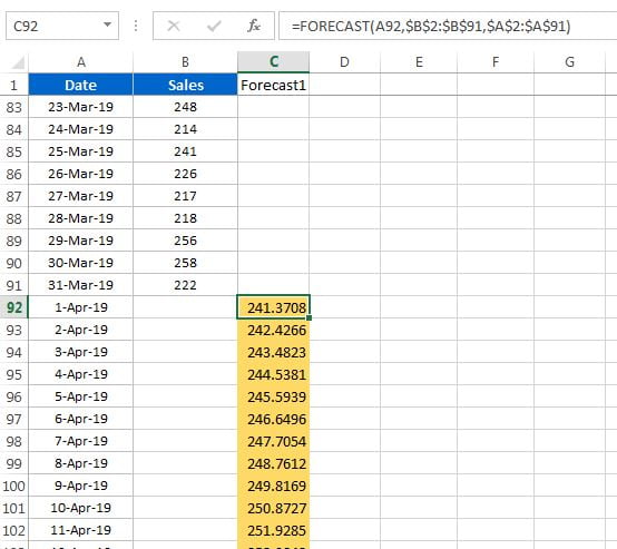
We have used forecast formula to do the forecasting for 1st APR’19 till 30th APR’19. Below is the Syntax of Forecast formula
Syntax
FORECAST(x, known_y's, known_x's)
The FORECAST function syntax has the following arguments:
- X: The data point for which you want to predict a value.
- Known_y’s : Required. The dependent array or range of data.
- Known_x’s: Required. The independent array or range of data.
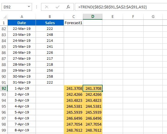
Trend formula:
The TREND function returns values along a linear trend. It fits a straight line (using the method of least squares) to the array’s known_y’s and known_x’s. TREND returns the y-values along that line for the array of new_x’s that you specify.
Syntax
TREND( known_y's, [known_x's], [new_x's], [const] )
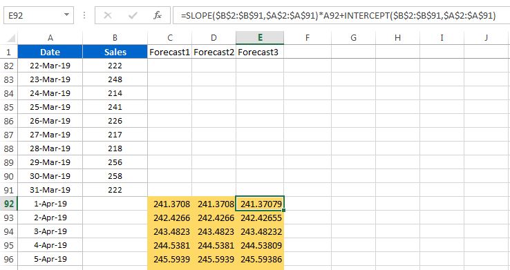
Linear regression equation using Excel formula:
We have used Excel formulas to get the foretasted sales using linear regression equation.
Linear Regression Equation Y = mx +c
Where x is an independent variable, Y is a dependent variable, m is the slope and c is intercept. So we have used excel formula Y = SLOPE * x + INTERCEPT
m  =SLOPE($B$2:$B$91,$A$2:$A$91)

c =INTERCEPT($B$2:$B$91,$A$2:$A$91)
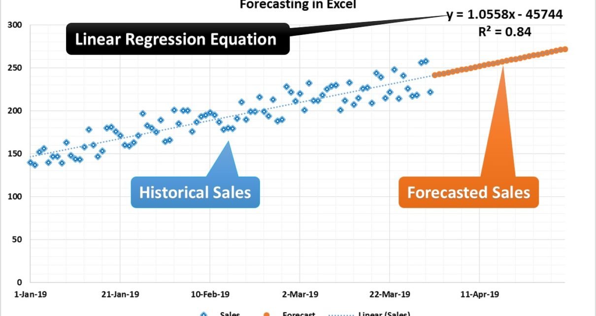
Linear regression equation using Excel Chart:
Just create the scatter chart or line chart for Actual sales data and add a linear regression trend line and check the Display Equation on the chart and Display R-squired value on the chart. Now Equation and R-squired value will be available on the chart.
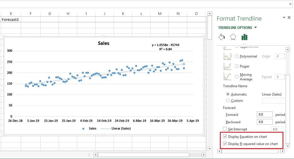
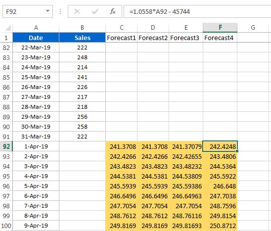
Copy the equation and put in the excel cell and change the x value with cell reference like we have taken below-
=1.0558*A92 – 45744
Click here to download this practice file.
Watch the step by step video tutorial:
Visit our YouTube channel to learn step-by-step video tutorials