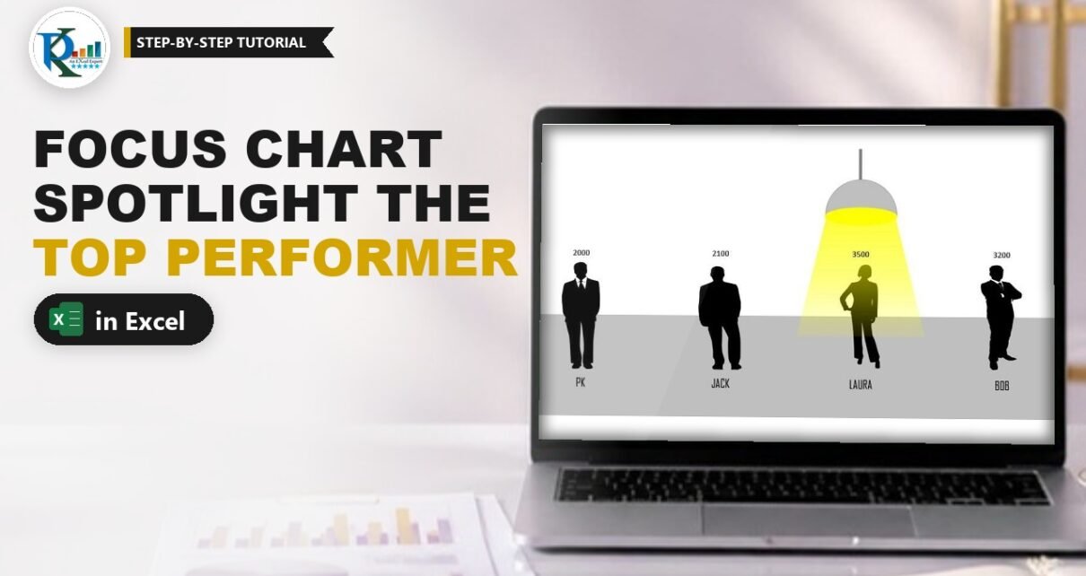
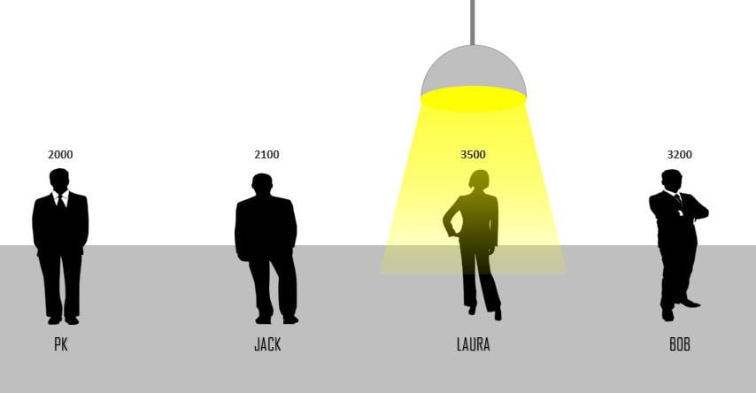
A focus chart in Excel puts a spotlight on your top performer, literally. Each team member stands as a silhouette on the chart, and a hanging lamp shines on whoever has the highest sales. Change any number and the lamp moves to the new leader on its own. PK builds it with one IF and MAX formula, a combo chart and a few shapes, with no VBA at all. It works well on a sales dashboard or a team review slide, where you want the winner to be obvious at a glance.
Watch the Video Tutorial
In the video PK adds two helper columns, builds the column and line combo chart, draws the hanging lamp from four shapes, fills the bars with people silhouettes and links the data labels to the sales figures.
What You Will Build
- A four-person sales table with two helper columns: Image Size and Hanging Light.
- An IF and MAX formula that finds the top performer automatically.
- A combo chart: picture-filled columns plus one line marker that carries the lamp.
- A hanging lamp made from a Pie, an Oval, a Trapezoid with a fading yellow gradient, and a Line.
- Data labels that show real sales numbers above each person.
Part 1: Set Up the Focus Chart Data
Step 1: Enter the sales table
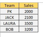
Type Team in A1 and Sales in B1, then the four names and their sales in A2:B5. In the post’s example the values are PK 2000, Jack 2100, Laura 3500 and Bob 3200. Turn off gridlines from the View tab so the chart sits on a clean page.
Step 2: Add the Image Size column
Type Image Size in C1 and enter 5 in C2:C5. These equal values become the bars, so every silhouette is drawn at the same height whatever the sales are. The sales numbers only appear in the labels.
Step 3: Add the Hanging Light formula
Type Hanging Light in D1, enter this formula in D2 and fill it down to D5:
=IF(B2=MAX($B$2:$B$5),C2*130%,NA())How the formula works
MAX($B$2:$B$5)finds the highest sales value. The range is locked with$so it stays the same as you fill down.B2=MAX(...)is TRUE only on the top performer’s row.C2*130%returns 6.5, which places the lamp 30% above the top of a 5-unit bar.NA()returns#N/Aon every other row. Charts skip#N/A, so only one marker is plotted.
Test it: change one sales value to the largest number and watch 6.5 jump to that row.
Part 2: Build the Combo Chart
Step 4: Insert a clustered column chart
Select A1:A5, hold Ctrl and select C1:D5, so the Sales column is skipped. Go to Insert › Charts › 2-D Clustered Column.
Step 5: Turn Hanging Light into a line with markers
Right-click any series and choose Change Series Chart Type. Set Hanging Light to Line with Markers and click OK. You now see one marker above the top performer’s column.
Step 6: Fix the axis and clean up
Right-click the vertical axis, choose Format Axis and set Minimum = 0 and Maximum = 10. A fixed maximum keeps the lamp at the same height whatever value is on top. Make the chart a little bigger, then delete the vertical axis, the gridlines, the legend and the chart title. Format the horizontal axis with Shape Outline › No Outline and make the names bold, larger and black.
Part 3: Draw the Hanging Lamp
Step 7: Build the lamp from four shapes
- Shade: Insert › Shapes › Basic Shapes › Pie. Drag the two yellow handles until it becomes a semicircle. Fill it grey and give it a darker grey outline.
- Bulb: Insert an Oval under the shade, fill it yellow, no outline.
- Light beam: Insert a Trapezoid, drag its yellow handle to widen the base, and set No Outline. In Format Shape › Fill choose Gradient fill, Linear, angle 90°. Remove one stop to leave three, put the middle stop at 50%, and colour all three yellow. Set the transparency to 20%, 50% and 90% so the beam fades as it falls.
- Cord: Insert a Line above the shade, colour it the same grey and set the weight to about 2.25 pt.
Select all four shapes, right-click and choose Group.
Step 8: Paste the lamp onto the marker
Copy the grouped lamp with Ctrl+C, click the Hanging Light marker in the chart and press Ctrl+V. The lamp replaces the marker and will move with it.
Part 4: People Pictures and Labels
Step 9: Fill each bar with a silhouette
PK took free vector silhouettes from Pixabay (search business people, vector graphics) and cropped one figure per person. Copy a picture, click the bars once, then click again on a single bar so only that bar is selected, and press Ctrl+V. Repeat for each person, using a female figure where it fits, as for Laura.
Next, select the columns, right-click and choose Add Data Labels. They show 5, because the bars come from Image Size. Open Format Data Labels, tick Value From Cells, select the Sales range B2:B5, click OK and untick Value. Make the labels bold, larger and black.
In Excel 2010 or earlier there is no Value From Cells option. Select one label, type = in the formula bar, click that person’s sales cell and press Enter. Repeat for each label.
Step 10: Test it
Lower the current leader’s sales and the lamp jumps to the person with the next-highest number. With the example data, drop Laura from 3,500 to 1,500 and the light moves to Bob at 3,200. Raise her to 5,000 and it swings back to her. PK runs the same test in the video.
Common Errors and Fixes
These fixes are general guidance based on how the chart is built.
Lamps appear on every person
The formula returns 0 or blank instead of NA(), so every row gets a marker. Use NA() as the value-if-false.
The lamp sits at a different height each time
The vertical axis is on Auto. Set the maximum to a fixed 10.
The lamp does not move when sales change
The MAX range is not locked. Check that it reads $B$2:$B$5 in every row, or extend it if you added people.
All bars show the same picture
The picture was pasted while the whole series was selected. Click once for the series and once more for the single bar before you paste.
Tips
- Need more people? Add rows, extend both helper columns, and widen the MAX range to match.
- To spotlight the lowest value instead, for example the person who needs coaching, swap
MAXforMINin the formula (our variation, not in the video). - Use transparent PNG silhouettes so the chart background shows through around each figure.
- Keep the lamp group narrow so the beam covers one person and not the neighbours.
- Microsoft’s page on the NA function explains why charts skip
#N/Avalues.
Want It Ready-Made?
Prefer to start from the finished file? The Innovation: Focus Chart in Excel template is available on NextGenTemplates.com, along with more Excel chart templates. If you want to build charts like this for your own dashboards, the Excel Pivot Tables & Dashboards course on NextGenTemplates Academy covers charts, infographics and dashboard design.
Related Tutorials
- Dynamically Highlight the Topper Student in a Chart
- Highlight a Specific Data Point in a Line Chart Dynamically
- Infographics with a Column Chart (Part 1)
- An Innovative Chart for Team-Level Performance
Frequently Asked Questions
What is a focus chart in Excel?
It is a column chart with picture-filled bars where a hanging lamp shines on the top performer. A helper column returns a value only for the highest number, and that single point carries the lamp, so the light moves by itself when the data changes.
How does the lamp know where to go?
The Hanging Light column uses IF with MAX. Only the row that equals the largest sales value gets a number, which is the image size multiplied by 130%. Every other row returns the NA error, which Excel charts do not plot, so there is only one marker for the lamp.
What happens if two people have the same top sales?
Both rows equal the maximum, so both get a marker and both show a lamp. If you want only one, add a tie-breaker in the sales column or limit the formula to the first match.
Why do the data labels show 5 instead of sales?
The bars are plotted from the Image Size column, which is 5 for everyone. Use Value From Cells in Format Data Labels and pick the Sales range, then untick Value, as shown in Step 9.
Can I use this chart in Excel 2010?
Yes. The formula, shapes and picture fills all work. Only Value From Cells is missing, so link each data label to its sales cell through the formula bar instead.
Where can I get the people images?
PK used free vector silhouettes from Pixabay, searched as business people. Any transparent PNG works, so you can pick male and female figures to match each team member.
About the Author
PK is a Microsoft Excel expert and trainer and the founder of PK: An Excel Expert and NextGenTemplates.com. He has been teaching Excel, VBA, Power Query and Power BI since 2016 on his YouTube channel.
Conclusion
The focus chart in Excel turns a plain sales comparison into a small story: four people on a stage and a lamp that always finds the leader. The engine is one formula, IF with MAX and NA, feeding a single line marker that carries the lamp, while equal-height columns hold the silhouettes. Build it once, swap in your own names and pictures, and your top performer will always be in the spotlight.