Comparison Infographic in Excel: Team vs Team Balance Chart

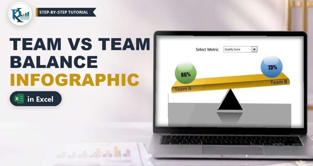
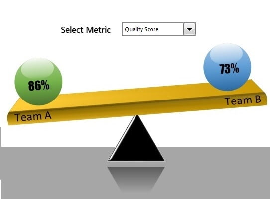
A comparison infographic in Excel turns a dry Team A vs Team B table into a see-saw: two 3D balls sit on a golden beam, and the beam tilts towards the team with the higher score. Pick a metric from a drop-down – AHT, Sales, Calls Handled, Quality Score and more – and the numbers, their format and the tilt all update. In this tutorial you build it with a Form Control combo box, INDEX formulas, conditional formatting, a few 3D shapes and one line of VBA that rotates the beam. It makes team performance reviews instantly readable.

Watch the Video Tutorial

In the video, PK builds the balance chart from scratch: the data sheet, the metric drop-down, the formulas, the 3D beam and balls, and the short macro that rotates the beam.

What You Will Build

• A metric drop-down (Form Control combo box) listing seven KPIs.
• Lookup formulas that pull Team A and Team B scores for the selected metric.
• Automatic number or percentage formatting driven by a Number Format column.
• A 3D balance: black triangle stand, golden beam and glossy green and blue balls.
• A one-line VBA macro that tilts the beam by up to 25 degrees according to the difference.

Part 1 – The Data Sheet

Step 1: Lay out the metrics

On a sheet named Data1, enter the table in A1:D8 with the headers Metrics, Team-A, Team-B and Number Format:

Metrics            Team-A   Team-B   Number Format
AHT                700      543      Number
Sales              34       54       Number
Calls Handles      100      110      Number
Quality Score      86%      73%      Percentage
Sales Conversion   34%      49%      Percentage
Productivity       78%      55%      Percentage
Escalations        4        4        Number

The Number Format column is the trick that later lets one cell show 700 for AHT and 86% for Quality Score. In the video the rows are also set to a height of 50 for readability.

Part 2 – The Drop-Down and the Formulas

Step 2: Insert the combo box

Add a new sheet named Chart1 and turn off gridlines on the View tab. Go to Developer > Insert > Combo Box (Form Control) and draw it near the top. Add a Select Metric label next to it with a text box or WordArt.

Right-click the combo box, choose Format Control and set:

• Input range: Data1!$A$2:$A$8 (the seven metrics)
• Cell link: $H$1

A Form Control combo box returns the position of the chosen item, so picking Sales puts 2 in H1. If you don’t see the Developer tab, enable it in File > Options > Customize Ribbon.

Step 3: Pull the scores with INDEX

Type Team A in C6 and Team B in D6, then enter:

C7  =INDEX(Data1!B2:B8,Chart1!H1)
D7  =INDEX(Data1!C2:C8,Chart1!H1)
B7  =INDEX(Data1!D2:D8,Chart1!H1)

INDEX returns the value at the row number held in H1. C7 and D7 are the two scores; B7 returns the word Number or Percentage for the selected metric.

Step 4: Format numbers and percentages automatically

If you simply format C7:D7 as a percentage, AHT turns into 70000%. Instead, select C7:D7 and add two rules with Home > Conditional Formatting > New Rule > Use a formula to determine which cells to format:

=$B$7="Number"       Format: Number, 0 decimal places
=$B$7="Percentage"   Format: Percentage, 0 decimal places

Now Quality Score shows 86% and AHT shows 700. Make the font of B7 white to hide the helper text.

Step 5: Build display text for the balls

Text boxes linked to cells ignore conditional formatting and would show 0.86. So create text versions of the scores:

C9  =TEXT(C7,IF($B$7="Percentage","0%","0"))
D9  =TEXT(D7,IF($B$7="Percentage","0%","0"))

How the formula works

• IF($B$7="Percentage","0%","0") picks a format code based on the metric type.
• TEXT(C7, ...) converts the score into text using that code, so 0.86 becomes 86% and 700 stays 700.
• $B$7 is locked with F4 so the formula can be copied from C9 to D9.

Part 3 – Draw the Comparison Infographic Shapes

Step 6: The triangle stand

Insert a Triangle from Basic Shapes. Fill it black with no outline, apply Shape Effects > Preset > Preset 5, then remove the shadow via Shape Effects > Shadow > No Shadow.

Step 7: The golden beam

1. Insert a Rectangle across the top of the triangle. Fill Gold, Accent 4, Darker 25%, no outline.
2. Right-click > Format Shape > Effects > 3-D Rotation and choose the preset Perspective Relaxed.
3. In 3-D Format set the Top bevel to Circle and its height to 20 pt for a thick, polished edge.

Step 8: The glossy balls

1. Insert an Oval (hold Shift for a circle), no outline, and use Fill > Gradient fill with a green preset gradient.
2. Insert a smaller oval in the upper part for the shine, no outline, gradient fill from the same preset family.
3. Remove the third gradient stop, set the second stop’s transparency to 30% and the last stop’s to 100%. This fades the highlight into the ball.
4. Select both ovals and Group them. Copy the group for Team B and switch the big oval to a blue preset gradient (repeat the shine settings).

Step 9: Link the labels

Insert a text box on each ball, click it, type = in the formula bar and click C9 (Team A) or D9 (Team B). Set Shape Fill and Outline to none and format the font. Add two more text boxes on the beam linked to C6 and D6, so renaming a team in the cell renames it on the chart.

Step 10: Group the moving parts

Select the beam, both balls and all four text boxes – but not the triangle – and choose Group. Note the group’s name in the Name Box (in the video it is Group 12); the macro needs it.

Part 4 – Rotate the Beam with VBA

Step 11: Calculate the tilt angle

In E7 enter:

E7  =(D7-C7)/D7*25

This is the percentage difference between the teams multiplied by 25. A positive result rotates the group clockwise, so the right side (Team B) goes down when Team B scores higher; a negative result tips it towards Team A. The factor 25 keeps the tilt small, because a rotation beyond 20-25 degrees looks unrealistic. For Calls Handles (100 vs 110) E7 returns about 2.27 degrees.

Step 12: Write the macro

Press Alt+F11, insert a module and add:

Sub Rotate_1()
    Sheet4.Shapes("Group 12").Rotation = Sheet4.Range("E7").Value
End Sub

Sheet4 is the code name of the Chart1 sheet in the video’s workbook (see it in the Project Explorer). Use your own sheet’s code name and your own group name from the Name Box.

Step 13: Assign the macro to the combo box

Right-click the combo box, choose Assign Macro and pick Rotate_1. Every time you choose a metric, the formulas update and the macro tilts the beam. Save the file as a macro-enabled workbook (the video uses .xlsb; .xlsm works too).

Common Errors and Fixes

The fixes and formula guards in this section are additions, not shown in the video.

Run-time error: The item with the specified name wasn’t found

The group name in the code doesn’t match. Select the group, read its name in the Name Box, and update Shapes("..."). You can also rename it in the Name Box to something clear, such as Balance.

The beam spins much too far

When one score is far smaller than the other, the formula can return a large angle. Cap it between -25 and 25 degrees, and stop a zero Team B score from causing #DIV/0!:

E7  =IFERROR(MAX(-25,MIN(25,(D7-C7)/D7*25)),0)

Ball shows 0.86 instead of 86%

The text box is linked to C7 instead of C9. Link it to the TEXT formula cell.

Nothing moves when I change the metric

Macros are disabled or not assigned. Enable content when you open the file and check that Rotate_1 is assigned to the combo box.

Tips

• Use the same balance for any two-way comparison: two regions, two products, this year vs last year.
• For lower-is-better metrics such as AHT or Escalations, remember the heavier side is the worse team; add a note or swap the sign for those rows.
• Keep the Data1 sheet as the only place you edit numbers; the chart sheet just reads it.
• Microsoft’s guide to adding a list box or combo box to a worksheet explains the Format Control options.

Want It Ready-Made?

If you want the finished, macro-enabled balance chart with all shapes and formulas in place, get the Comparison Infographics in Excel template on NextGenTemplates.com, or browse more Charts and Visualization templates. To build interactive charts, infographics and dashboards with confidence, join the course Excel Pivot Tables and Dashboards on NextGenTemplates Academy.

Related Tutorials

• Dynamic Comparison in Butterfly Chart
• Team Comparison with Tornado or Butterfly Charts in Excel
• Stylish and Dynamic Comparison Chart
• Excel Form Controls: Combo Box, Spin Button and Option Buttons
• Beautiful 3D Visualization in Excel

Frequently Asked Questions

How do I compare two teams visually in Excel?

Pull both scores for a selected metric with INDEX, show them on two shapes, and tilt a grouped beam with a small macro based on the percentage difference. The heavier side is the team with the higher score.

Can I build this comparison infographic without VBA?

The scores, labels and formats update with formulas alone, but rotating a shape needs the one-line macro. Without it the balance stays level.

Why does the combo box return a number?

A Form Control combo box always returns the position of the selected item. INDEX uses that position to fetch the matching row.

How do I show some metrics as numbers and others as percentages?

Store the format type in a column, use conditional formatting on the score cells, and use TEXT with IF for the text boxes on the balls.

How much should the beam rotate?

The video multiplies the percentage difference by 25, so small gaps give a gentle tilt. Keep the maximum at about 20 to 25 degrees so the chart still looks natural.

About the Author

PK is a Microsoft Excel expert and trainer and the founder of PK: An Excel Expert and NextGenTemplates.com. He has been teaching Excel, Power Query and Power BI since 2016 on his YouTube channel.

Conclusion

This comparison infographic in Excel combines a combo box, INDEX, conditional formatting, TEXT, a few 3D shapes and one line of VBA into a balance that anyone can read at a glance. Choose a metric and the heavier team sinks. Build it once, point it at your own KPIs, and your next team review will be far more engaging than a table of numbers.